
Mature Functions: Programmed Ferroptosis
1 Preprocessing
The default GEO data file is located at C:/GEOANALYSIS/GSE232429.
Change the working directory in R to: C:/GEOANALYSIS/GSE232429.
Highly recommended to use Rstudio. Need to select the environment which containing anndata, in Tools > Global options > Python > Python interpreter
######Mature Functions: Programmed Ferroptosis ########################
####1 Preprocessing####
#The default GEO data file is located at C:/GEOANALYSIS/GSE232429.
#Change the working directory in R to: C:/GEOANALYSIS/GSE232429.
#Highly recommended to use Rstudio. Need to select the environment which containing anndata, in Tools > Global options > Python > Python interpreter

###1.1 Load required packages for this section (R Studio)###############
library(Seurat)
library(multtest)
library(dplyr)
library(ggplot2)
library(patchwork)
library(tidyverse)
library(future)
library(harmony)
library(RColorBrewer)
library(ggrepel)
library(sceasy)

###1.2 Create vector to read files (R)Permalink###############
#Database download link:  https://biocomputing.cowtransfer.com/s/2df0081e282147
#Password: ufurmd
setwd("C:/GEOANALYSIS/GSE2324291w")

## Save the file names in the folder to "dir_name"
dir_name <- list.files("./data")
## check "dir_name"
dir_name
#[1] "MCAO1" "MCAO2" "Sham1"
## Assign names to "dir_name" based on folder names
names(dir_name) <- c("MCAO1", "MCAO2", "Sham1")
## Check the "dir_name" after name assignment
print(dir_name)
# Model1   Model2   Treat1   Treat2
#"Model1" "Model2" "Treat1" "Treat2"

#File Structure
# ---[C:\]
#   ---[GEOANALYSIS]
#     ---[GSE232429]
#        ---[data]
#          ---[Sham1]
#             ---matrix.mtx.gz
#             ---features.tsv.gz
#             ---barcodes.tsv.gz
#          ---[MCAO1]
#             ---matrix.mtx.gz
#             ---features.tsv.gz
#             ---barcodes.tsv.gz
#           ---[MCAO2]
#             ---matrix.mtx.gz
#             ---features.tsv.gz
#             ---barcodes.tsv.gz
#        ---[figures]
#        ---[output]
#        ---[saves]


###1.3 Read data and create Seurat objects with sample names (R)###############
## Initialize a list for Seurat objects
scRNAlist <- list()

## Loop through each sample, read data, and create Seurat objects
for (sample in names(dir_name)) {
  # Construct the full path to the data directory
  data_path <- file.path("./data", dir_name[sample])

  # Read 10X data and create a Seurat object [to filter out cells with fewer than 200 genes (min.features = 200) and genes covered by fewer than 3 cells (min.cells = 3)]
  counts <- Read10X(data.dir = data_path)
  obj <- CreateSeuratObject(counts,
                            project = sample,
                            min.cells = 3,
                            min.features = 200)

  # Overwrite orig.ident to ensure it is the folder name
  obj$orig.ident <- sample

  # Save to list
  scRNAlist[[sample]] <- obj

  # Output sample name for confirmation
  cat(paste("Processed sample:", sample, "\n"))
}

###1.4 Filter the data###############
#Calculate the ratio of mitochondria to red blood cells
for(i in 1:length(scRNAlist)){
  sc <- scRNAlist[[i]]
  # Calculation of mitochondrial ratio
  sc[["mt_percent"]] <- PercentageFeatureSet(sc, pattern = "^mt-")
  # Calculate the red blood cell ratio
  HB_genes <- c("Hbb-bt", "Hbb-bs", "Hbb-bh2", "Hbb-bh1", "Hbb-y", "Hba-x", "Hba-a1", "Hbq1b", "Hba-a2", "Hbq1a")
  # Make sure the gene name exists in the data
  HB_genes <- intersect(HB_genes, rownames(sc))
  if (length(HB_genes) == 0) {
    stop("No red blood cell-related genes were found in the dataset. Please check that the gene names are correct!")
  }
  HB_m <- match(HB_genes, rownames(sc@assays$RNA))
  HB_genes <- rownames(sc@assays$RNA)[HB_m]
  HB_genes <- HB_genes[!is.na(HB_genes)]
  sc[["HB_percent"]] <- PercentageFeatureSet(sc, features=HB_genes)
  # Assign sc to scRNAlist[[i]]
  scRNAlist[[i]] <- sc
  # Delete sc
  rm(sc)
}

#Merge and then create a quality control chart
#MCAO1, MCAO2, and Sham1 are merged to generate CI
CI <- merge(scRNAlist[[1]], y = scRNAlist[-1], add.cell.ids = names(scRNAlist))
head(colnames(CI))
unique(sapply(X = strsplit(colnames(CI), split = "_"), FUN = "[", 1))
Idents(CI) <- "orig.ident"

plot1 <- FeatureScatter(CI, feature1 = "nCount_RNA", feature2 = "mt_percent", raster=FALSE)
plot2 <- FeatureScatter(CI, feature1 = "nCount_RNA", feature2 = "nFeature_RNA", raster=FALSE)
p1 <- CombinePlots(plots = list(plot1, plot2))#QC plot 1
p2 <- VlnPlot(CI, features = c("mt_percent", "nFeature_RNA", "nCount_RNA", "HB_percent"), ncol = 4, pt.size=0)#QC plot 2
p3 <- VlnPlot(CI, features = c("mt_percent", "nFeature_RNA", "nCount_RNA", "HB_percent"), ncol = 4, pt.size=0.5)#QC plot 3

#Output QC plots into "figures" fold
ggsave(filename = "./figures/QC Plot1.pdf", plot = p1, device = 'pdf', width = 24, height = 12, units = 'cm')
ggsave(filename = "./figures/QC Plot2.pdf", plot = p2, device = 'pdf', width = 35, height = 15, units = 'cm')
ggsave(filename = "./figures/QC Plot3.pdf", plot = p3, device = 'pdf', width = 35, height = 15, units = 'cm')

###1.5 Remove cells with high mitochondrial gene expression or extreme values (R)###############
# nFeature_RNA: Genes expressed in each cell > 500 and < 8000;
# nCount_RNA: Retain cells with nCount_RNA values below the 98th percentile.
# mt_percent: Mitochondrial gene expression < 30% of total gene expression;
# HB_percent: The percentage of gene expression in erythrocytes <5%
scRNAlist <- lapply(X = scRNAlist, FUN = function(x){
  x <- subset(x,
              subset = nFeature_RNA > 500 & nFeature_RNA < 8000 &
                mt_percent < 30 &
                HB_percent < 5 &
                nCount_RNA < quantile(nCount_RNA,0.98))})

###1.6 Data integration using the harmony function, generating `testAB.integrated`.###
#Merge seurat objects
scRNAlist <- merge(scRNAlist[[1]], y = scRNAlist[-1], add.cell.ids = names(scRNAlist))

#Screening for highly variable genes and dimensionality reduction
scRNAlist <- NormalizeData(scRNAlist) %>%
  FindVariableFeatures(selection.method = "vst",nfeatures = 3000) %>%
  ScaleData() %>%
  RunPCA(npcs = 30, verbose = T)

#integrating
testAB.integrated <- RunHarmony(scRNAlist, group.by.vars = "orig.ident")

###1.7 Add sample and group information (R)Permalink############
# Copy orig.ident to Sample
testAB.integrated@meta.data$Sample <- testAB.integrated@meta.data$orig.ident

# Copy orig.ident to Group, removing the numbers
testAB.integrated@meta.data$Group <- gsub("[0-9]", "", testAB.integrated@meta.data$orig.ident)

# Check the modified metadata
head(testAB.integrated@meta.data)

###1.8 Clustering and dimensionality reduction using UMAP/t-SNE###################
#The Seurat object generated after clustering is defined as NeuronR1.
#"NeuronR1" was used for the first round of cell state classification (Round 1).
NeuronR1 <- FindNeighbors(testAB.integrated, reduction = "harmony", dims = 1:15) %>%
  FindClusters(resolution = 0.1)

#Dimensionality reduction
NeuronR1 <- RunTSNE(NeuronR1, reduction = "harmony", dims = 1:10)
NeuronR1 <- RunUMAP(NeuronR1, reduction = "harmony", dims = 1:30)

###1.10 Data oreoricessing is completed, export data####################
##1.10.1 Export Seurat object "NeuronR1" into "saves" fold
save(NeuronR1, file = "./saves/NeuronR1.Rdata")

##1.10.2 Export seurat object "Neuron R1" as a h5ad file for Section 2.
#Export the cells and 3000 highly variable genes in h5ad format.
# Create a new folder
dir.create("./output/h5adfile", recursive = TRUE, showWarnings = FALSE)
# Define a general export function (to export highly variable genes)
export_high_var_to_h5ad <- function(seurat_obj, filename, top_n = 3000) {
  # Set Assay
  DefaultAssay(seurat_obj) <- "RNA"
  seurat_obj[["RNA"]] <- as(seurat_obj[["RNA"]], Class = "Assay")  # Convert Assay5 type to Assay4

  # Find highly variable genes
  seurat_obj <- FindVariableFeatures(seurat_obj, selection.method = "vst", nfeatures = top_n)
  high_var_genes <- VariableFeatures(seurat_obj)

  # Construct a new object containing only highly variable genes.
  seurat_high_var <- subset(seurat_obj, features = high_var_genes)

  # Export path
  out_path <- file.path("output/h5adfile", filename)

  # Convert the format and save.
  sceasy::convertFormat(
    seurat_high_var,
    from = "seurat",
    to = "anndata",
    outFile = out_path
  )
  cat("Highly variable genes have been successfully exported:", out_path, "\n")
}

# Export h5ad
export_high_var_to_h5ad(NeuronR1, "NeuronR1.h5ad")
H5ad saved as NeuronR1.h5ad, change it to GSE232429 Neuron.h5ad
Save the variable table as Round0.Rdata. OR: Do not close R to ensure the subsequent programs can run.
Round 1
2 𝙄𝙙𝙚𝙣𝙩𝙞𝙛𝙮 𝙘𝙚𝙡𝙡𝙨 𝙪𝙣𝙙𝙚𝙧𝙜𝙤𝙞𝙣𝙜 𝙥𝙧𝙤𝙜𝙧𝙖𝙢𝙢𝙚𝙙 𝙛𝙚𝙧𝙧𝙤𝙥𝙩𝙤𝙨𝙞𝙨.
Start
2.1 𝐒𝐭𝐞𝐩 𝟏: 𝐀𝐜𝐭𝐢𝐯𝐚𝐭𝐞 𝐮𝐬𝐢𝐧𝐠 𝐭𝐡𝐞 𝐩𝐫𝐨𝐱𝐢𝐦𝐢𝐭𝐲 𝐦𝐞𝐭𝐡𝐨𝐝. (Python)
Import GSE232429 Neuron.h5ad into [LittleSnowFox's Anaconda installation directory]\database\Tracing_sample\Nerveferroptosis\data\.
import numpy as np
import os
import LittleSnowFox as kl

print(kl.__version__)
kl.kl_initialize(0)
parent_directory_origin = kl.kl_settings.parent_directory_origin
print(parent_directory_origin)

current_folder = kl.workcatalogue.choosemode_kl(parent_directory_origin,'Lineage',1)
print(current_folder)
current_folder = kl.workcatalogue.choosemode_kl(parent_directory_origin,'Lineage',1)
print(current_folder)

#选择要使用哪个样本
choosen_sample = "Nerveferroptosis"

#选择.h5ad文件
h5ad_filename = "GSE232429 Neuron.h5ad"


#运行自带的示例,并获取稀疏矩阵
#这里需要做非示例的函数进去
current_folder_input = current_folder


orig_adata,loading_directory,distance_matrix = kl.preprocessing.kl_dense_matrix_sample(
    choosen_sample,
    h5ad_filename,
    "draw",
    current_folder_input,
    round_of_smooth=1,
    neighbor_N=13000,
    beta=0.1,
    truncation_threshold=0.001,
    save_subset=True,
    use_existing_KNN_graph=False,
    compute_new_Smatrix=True,
    use_full_Smatrix = True,
    )
#orig_adata,loading_directory,distance_matrix_sparse = kl.preprocessing.kl_dense_matrix_sample(choosen_sample,h5ad_filename,"draw",current_folder_input)

#运行自带的示例,并获取非稀疏矩阵
#这里需要做非示例的函数进去
#current_folder_input = current_folder
#loading_directory,distance_matrix = kl.preprocessing.kl_dense_matrix(choosen_sample,h5ad_filename,"draw",current_folder_input)

orig_adata.obs['orig.ident']
orig_adata

#需要区分dense和sparase
save_list = ["orig_adata.obs['orig.ident']", "orig_adata.obsm['X_umap']"]

import scipy.sparse
distance_matrix_sparse = scipy.sparse.csr_matrix(distance_matrix)

#将要计算的文件保存到/result
merged_csv,result_directory = kl.workcatalogue.kl_save(loading_directory,choosen_sample,distance_matrix_sparse,save_list,orig_adata)
2.2 𝐒𝐭𝐞𝐩 𝟐: 𝐔𝐬𝐞 𝐮𝐧𝐬𝐮𝐩𝐞𝐫𝐯𝐢𝐬𝐞𝐝 𝐥𝐞𝐚𝐫𝐧𝐢𝐧𝐠. (Matlab)
Afterward, execute the following file:
[LittleSnowFox's Anaconda installation directory]\database\Tracing_sample\Nerveferroptosis\main_v3_matlab_run_me.m
%% Load data and Split to compute
%% Load data and Split to compute
MM0 = load('./result/distance_matrix.mat');
MM0 = MM0.distance_matrix;

%% 读取要排序的对象
count_=readtable('./result/merged_data.csv');

%% 得到边界划分点
[p,splitlist] = binary_corr_sorting(MM0,20,300,5,5);

%% 对划分点去重
[uniqueList, ~, ~] = unique(splitlist, 'stable');

%% 对相似度矩阵排序
MM=MM0(p,p);
split=[];

%% 重排count_result
count_result=count_(p,:);
split_simple=uniqueList;

%% 第一个起始位点置为1
split_simple(1)=1;
split_simple=[split_simple,length(MM0)];

%% 计算均值矩阵
[simple_matrix]=sample_computing(count_result,split_simple,MM,"mean");


%% 合并成小矩阵
ClusterReslut=cluster_map(split_simple,simple_matrix,0,0.0002,0);
count_result.Result = ClusterReslut;


%重排小矩阵
[cluster_map_matrix] = genetic_encoder( ...
    simple_matrix, ...
    60, ...% nPop = 50;  % 种群规模大小为30
    1, ...% nPc = 1; % 子代规模的比例0.8
    200, ...% maxIt = 200; % 最大迭代次数
    5 ...% cycletimes = 200; % 循环计算次数
    );


%重拍小矩阵方案2
% 创建行和列标签(示例)
%row_labels = cluster_map_label;
%column_labels = cluster_map_label;
% 使用 heatmap 函数并传递相应参数
h = heatmap(cluster_map_matrix);
%h.YDisplayLabels = row_labels; % 设置行标签
%h.XDisplayLabels = column_labels; % 设置列标签
h.ColorLimits = [0, 0.00007]

% %对小矩阵进行排序
% %计算pesudotime,两种计算模式,mean和median
% %疑问,pseudotime跟着小矩阵重排了吗?
% [pesudotime_info] = pesudotime_combine(split_simple,count_.Pst,"mean")
% %使用sigmoid函数处理伪时间
% pesudotime_info_sigmoid = sigmoid(pesudotime_info,45,10,100);
% %pesudotime_info_sigmoid = pesudotime_info;
% % 使用 heatmap 函数并传递相应参数
%
% number_of_length = 1:length(cluster_map_matrix);
%
% row_labels = pesudotime_info_sigmoid;
% column_labels = number_of_length;

figure(1)
hi = heatmap(cluster_map_matrix);
hi.ColorLimits = [0, 0.00002]


%% 临近法激活
writetable(count_result,"result/time_map.csv");

%临近法激活,()
corr_matrix = relevance_generate(0.00007,3,cluster_map_matrix);
heatmap(corr_matrix);

%% 编码
encode_result = encoder_corr_matrix(0.000071,0.000069,50,3,cluster_map_matrix);
figure(2)
hj = heatmap(encode_result);

%% 解码
figure(3)
[weighting_decode,decode_result] = decoder_corr_matrix(encode_result);
weighting_result = weighting_decode + decode_result;
hk = heatmap(weighting_result);
hk.ColorLimits = [40, 50]
Group result generated in [LittleSnowFox's Anaconda installation directory]\database\Tracing_sample\Nerveferroptosis\result\time_map.csv.
2.3 𝐒𝐭𝐞𝐩 𝟑: 𝐏𝐞𝐫𝐟𝐨𝐫𝐦 𝐨𝐦𝐢𝐜𝐬 𝐚𝐧𝐚𝐥𝐲𝐬𝐢𝐬. (R)
Open variable table Round0.Rdata to continue. OR: You didn’t closed R Studio.
2.3.1 After analysis, import results from ‘1n13000_result.csv’ into metadata (R)
Place time_map.csv in the R working directory. File is usuallly located at C:/GEOANALYSIS/GSE232429w/
##2.4 Calculate the scores of ferroptosis and apoptosis in each cell population.
##2.4.1 Load required packages for this section (R Studio)############
library(Seurat)
library(multtest)
library(dplyr)
library(ggplot2)
library(patchwork)
library(tidyverse)
library(UCell)
setwd("C:/GEOANALYSIS/GSE2324291w")
# ============================================
# Binary Scoring System with p-value Filter
# Only genes with p_val < 0.05 are scored
# No visualization - CSV outputs only
# ============================================
# ============================================
# Load DEG Results
# ============================================
cat("========== LOADING DEG RESULTS ==========\n")
R1_all_Table <- read.csv("./output/Round1/R1_all_Table.csv", row.names = 1)
R1_DEG=get(load(file = "./saves/Round1/R1_DEG.Rdata"))
cat(sprintf("Loaded %d DEG results\n", nrow(R1_all_Table)))
# ============================================
# Define Gene Signatures
# ============================================
# Ferroptosis genes - Promote ferroptosis when UPREGULATED
pro_ferroptosis_genes <- c(
"Acsl4", # Lipid peroxidation executor
"Ptgs2", # COX2, lipid peroxidation
"Alox15", # Lipoxygenase, lipid peroxidation
"Alox12", # Lipoxygenase, lipid peroxidation
"Lpcat3", # Lipid remodeling
"Tfrc", # Transferrin receptor, iron uptake
"Ncoa4", # Ferritinophagy, iron release
"Hmox1" # Heme degradation, iron release
)
# Ferroptosis genes - Inhibit ferroptosis when UPREGULATED
anti_ferroptosis_genes <- c(
"Gpx4", # Key ferroptosis inhibitor
"Slc7a11", # Cystine importer
"Aifm2", # FSP1
"Nfe2l2", # NRF2
"Gclc", # GSH synthesis
"Gclm", # GSH synthesis
"Gsr", # GSH recycling
"Fth1", # Ferritin, iron storage
"Ftl1", # Ferritin, iron storage
"Gss" # GSH synthesis
)
# Apoptosis genes - Promote apoptosis when UPREGULATED
pro_apoptosis_genes <- c(
"Bax", "Bak1", "Bid", # BCL2 family, pro-death
"Casp3", "Casp9", "Casp8", # Caspases
"Casp7", # Executioner caspase
"Apaf1", "Cycs", # Apoptosome
"Fas", "Trp53", "Fadd" # Death receptors, p53
)
# Apoptosis genes - Inhibit apoptosis when UPREGULATED
anti_apoptosis_genes <- c(
"Bcl2", "Bcl2l1", "Mcl1", # BCL2 family, pro-survival
"Xiap", "Birc2", "Birc3", # IAPs
"Hspb1" # HSP27
)
# ============================================
# Binary Scoring Function with p-value Filter
# ============================================
calculate_binary_score <- function(deg_table, cluster_name,
pro_genes, anti_genes,
pathway_name,
p_threshold = 0.05) {
# Filter for this cluster
cluster_data <- deg_table %>% filter(cluster == cluster_name)
# Initialize counters
total_score <- 0
detected_genes <- 0
significant_genes <- 0
pro_up_sig <- 0
pro_down_sig <- 0
anti_up_sig <- 0
anti_down_sig <- 0
gene_details <- data.frame(
gene = character(),
log2FC = numeric(),
p_val = numeric(),
score = integer(),
type = character(),
significant = logical(),
stringsAsFactors = FALSE
)
# Score PRO-death genes
for (gene in pro_genes) {
gene_data <- cluster_data %>% filter(gene == !!gene)
if (nrow(gene_data) > 0) {
log2fc <- gene_data$avg_log2FC[1]
pval <- gene_data$p_val[1]
if (!is.na(log2fc) && !is.na(pval)) {
detected_genes <- detected_genes + 1
# Only score if p_val < threshold
if (pval < p_threshold) {
significant_genes <- significant_genes + 1
if (log2fc > 0) {
score <- 1 # Upregulated pro-death gene = promotes death
pro_up_sig <- pro_up_sig + 1
} else {
score <- -1 # Downregulated pro-death gene = inhibits death
pro_down_sig <- pro_down_sig + 1
}
total_score <- total_score + score
is_sig <- TRUE
} else {
score <- 0 # Not significant, don't count
is_sig <- FALSE
}
gene_details <- rbind(gene_details, data.frame(
gene = gene,
log2FC = log2fc,
p_val = pval,
score = score,
type = "pro",
significant = is_sig
))
}
}
}
# Score ANTI-death genes
for (gene in anti_genes) {
gene_data <- cluster_data %>% filter(gene == !!gene)
if (nrow(gene_data) > 0) {
log2fc <- gene_data$avg_log2FC[1]
pval <- gene_data$p_val[1]
if (!is.na(log2fc) && !is.na(pval)) {
detected_genes <- detected_genes + 1
# Only score if p_val < threshold
if (pval < p_threshold) {
significant_genes <- significant_genes + 1
if (log2fc > 0) {
score <- -1 # Upregulated anti-death gene = inhibits death
anti_up_sig <- anti_up_sig + 1
} else {
score <- 1 # Downregulated anti-death gene = promotes death
anti_down_sig <- anti_down_sig + 1
}
total_score <- total_score + score
is_sig <- TRUE
} else {
score <- 0 # Not significant
is_sig <- FALSE
}
gene_details <- rbind(gene_details, data.frame(
gene = gene,
log2FC = log2fc,
p_val = pval,
score = score,
type = "anti",
significant = is_sig
))
}
}
}
return(list(
total_score = total_score,
detected_genes = detected_genes,
significant_genes = significant_genes,
pro_up_sig = pro_up_sig,
pro_down_sig = pro_down_sig,
anti_up_sig = anti_up_sig,
anti_down_sig = anti_down_sig,
gene_details = gene_details
))
}
# ============================================
# FERROPTOSIS ANALYSIS - Binary Scoring
# ============================================
cat("\n========== FERROPTOSIS BINARY SCORING (p < 0.05) ==========\n")
clusters <- unique(R1_all_Table$cluster)
ferroptosis_results <- list()
for (cluster_name in clusters) {
result <- calculate_binary_score(
R1_all_Table,
cluster_name,
pro_ferroptosis_genes,
anti_ferroptosis_genes,
"Ferroptosis",
p_threshold = 0.05
)
ferroptosis_results[[cluster_name]] <- result
}
# Create summary table
ferroptosis_summary <- data.frame(
CellGroupR1 = names(ferroptosis_results),
Ferroptosis_Final_Score = sapply(ferroptosis_results, function(x) x$total_score),
Total_Genes_Detected = sapply(ferroptosis_results, function(x) x$detected_genes),
Significant_Genes = sapply(ferroptosis_results, function(x) x$significant_genes),
Pro_Ferro_UP = sapply(ferroptosis_results, function(x) x$pro_up_sig),
Pro_Ferro_DOWN = sapply(ferroptosis_results, function(x) x$pro_down_sig),
Anti_Ferro_UP = sapply(ferroptosis_results, function(x) x$anti_up_sig),
Anti_Ferro_DOWN = sapply(ferroptosis_results, function(x) x$anti_down_sig),
stringsAsFactors = FALSE
) %>%
arrange(desc(Ferroptosis_Final_Score))
print(ferroptosis_summary)
# Save results
write.csv(ferroptosis_summary,
"./output/Round1/ferroptosis_binary_score_pval_filtered.csv",
row.names = FALSE)
# Save detailed gene information
ferroptosis_gene_details <- do.call(rbind, lapply(names(ferroptosis_results), function(cluster) {
details <- ferroptosis_results[[cluster]]$gene_details
if (nrow(details) > 0) {
details$CellGroupR1 <- cluster
return(details)
}
}))
write.csv(ferroptosis_gene_details,
"./output/Round1/ferroptosis_gene_details_with_pval.csv",
row.names = FALSE)
# ============================================
# APOPTOSIS ANALYSIS - Binary Scoring
# ============================================
cat("\n========== APOPTOSIS BINARY SCORING (p < 0.05) ==========\n")
apoptosis_results <- list()
for (cluster_name in clusters) {
result <- calculate_binary_score(
R1_all_Table,
cluster_name,
pro_apoptosis_genes,
anti_apoptosis_genes,
"Apoptosis",
p_threshold = 0.05
)
apoptosis_results[[cluster_name]] <- result
}
# Create summary table
apoptosis_summary <- data.frame(
CellGroupR1 = names(apoptosis_results),
Apoptosis_Final_Score = sapply(apoptosis_results, function(x) x$total_score),
Total_Genes_Detected = sapply(apoptosis_results, function(x) x$detected_genes),
Significant_Genes = sapply(apoptosis_results, function(x) x$significant_genes),
Pro_Apop_UP = sapply(apoptosis_results, function(x) x$pro_up_sig),
Pro_Apop_DOWN = sapply(apoptosis_results, function(x) x$pro_down_sig),
Anti_Apop_UP = sapply(apoptosis_results, function(x) x$anti_up_sig),
Anti_Apop_DOWN = sapply(apoptosis_results, function(x) x$anti_down_sig),
stringsAsFactors = FALSE
) %>%
arrange(desc(Apoptosis_Final_Score))
# Save results
write.csv(apoptosis_summary,
"./output/Round1/apoptosis_binary_score_pval_filtered.csv",
row.names = FALSE)
# Save detailed gene information
apoptosis_gene_details <- do.call(rbind, lapply(names(apoptosis_results), function(cluster) {
details <- apoptosis_results[[cluster]]$gene_details
if (nrow(details) > 0) {
details$CellGroupR1 <- cluster
return(details)
}
}))
write.csv(apoptosis_gene_details,
"./output/Round1/apoptosis_gene_details_with_pval.csv",
row.names = FALSE)
# ============================================
# COMBINED COMPARISON
# ============================================
cat("\n========== COMBINED COMPARISON ==========\n")
comparison_summary <- ferroptosis_summary %>%
select(CellGroupR1,
Ferroptosis_Final_Score,
Ferro_Sig_Genes = Significant_Genes) %>%
left_join(
apoptosis_summary %>%
select(CellGroupR1,
Apoptosis_Final_Score,
Apop_Sig_Genes = Significant_Genes),
by = "CellGroupR1"
) %>%
mutate(
Total_Death_Score = Ferroptosis_Final_Score + Apoptosis_Final_Score,
Dominant_Death_Mode = case_when(
Ferroptosis_Final_Score > Apoptosis_Final_Score + 2 ~ "Ferroptosis_Dominant",
Apoptosis_Final_Score > Ferroptosis_Final_Score + 2 ~ "Apoptosis_Dominant",
TRUE ~ "Mixed_Death"
)
) %>%
arrange(desc(Total_Death_Score))
cat("\nCombined Comparison (sorted by Total Death Score):\n")
print(comparison_summary)
write.csv(comparison_summary,
"./output/Round1/cell_death_binary_score_comparison_pval_filtered.csv",
row.names = FALSE)
# ============================================
# CONTINUOUS MODULE SCORING (AddModuleScore)
# ============================================
cat("\n========== CONTINUOUS MODULE SCORING (AddModuleScore) ==========\n")
# -------------------------------
# 1. Ferroptosis continuous score
# -------------------------------
cat("Calculating continuous Ferroptosis scores...\n")
# Positive (promoting ferrodeath) module
R1_DEG <- AddModuleScore(
object = R1_DEG,
features = list(pro_ferroptosis_genes),
name = "Pro_Ferro_Cont",
ctrl = min(100, length(pro_ferroptosis_genes)), # Control the number of genes to not exceed the list size.
seed = 123
)
# Negative (iron-suppressing death) module
R1_DEG <- AddModuleScore(
object = R1_DEG,
features = list(anti_ferroptosis_genes),
name = "Anti_Ferro_Cont",
ctrl = min(100, length(anti_ferroptosis_genes)),
seed = 123
)
# Sum Ferroptosis Potential Index (FPI)
R1_DEG@meta.data$Ferro_FPI_Cont <-
R1_DEG@meta.data$Pro_Ferro_Cont1 - R1_DEG@meta.data$Anti_Ferro_Cont1
# -------------------------------
# 2. Apoptosis continuous score
# -------------------------------
cat("Calculating continuous Apoptosis scores...\n")
R1_DEG <- AddModuleScore(
object = R1_DEG,
features = list(pro_apoptosis_genes),
name = "Pro_Apop_Cont",
ctrl = min(100, length(pro_apoptosis_genes)),
seed = 123
)
R1_DEG <- AddModuleScore(
object = R1_DEG,
features = list(anti_apoptosis_genes),
name = "Anti_Apop_Cont",
ctrl = min(100, length(anti_apoptosis_genes)),
seed = 123
)
R1_DEG@meta.data$Apop_FPI_Cont <-
R1_DEG@meta.data$Pro_Apop_Cont1 - R1_DEG@meta.data$Anti_Apop_Cont1
# -------------------------------
# 3. Summarize the mean and median of continuous ratings by group
# -------------------------------
cat("\nSummarizing continuous module scores by cluster...\n")
continuous_summary <- R1_DEG@meta.data %>%
group_by(CellGroupR1) %>%
summarise(
# Ferroptosis
mean_Pro_Ferro = mean(Pro_Ferro_Cont1, na.rm = TRUE),
mean_Anti_Ferro = mean(Anti_Ferro_Cont1, na.rm = TRUE),
mean_Ferro_FPI = mean(Ferro_FPI_Cont, na.rm = TRUE),
median_Ferro_FPI = median(Ferro_FPI_Cont, na.rm = TRUE),
# Apoptosis
mean_Pro_Apop = mean(Pro_Apop_Cont1, na.rm = TRUE),
mean_Anti_Apop = mean(Anti_Apop_Cont1, na.rm = TRUE),
mean_Apop_FPI = mean(Apop_FPI_Cont, na.rm = TRUE),
median_Apop_FPI = median(Apop_FPI_Cont, na.rm = TRUE),
n_cells = n()
) %>%
arrange(desc(mean_Ferro_FPI)) # Ferro FPI sorted in descending order
print(continuous_summary)
# Save summary table
write.csv(continuous_summary,
"./output/Round1/continuous_module_scores_summary.csv",
row.names = FALSE)
# -------------------------------
# 4. Comparison with binary scoring (merged table)
# -------------------------------
cat("\nMerging binary and continuous results for comparison...\n")
comparison_both <- ferroptosis_summary %>%
select(CellGroupR1, Ferroptosis_Final_Score, Ferro_Sig_Genes = Significant_Genes) %>%
left_join(
apoptosis_summary %>%
select(CellGroupR1, Apoptosis_Final_Score, Apop_Sig_Genes = Significant_Genes),
by = "CellGroupR1"
) %>%
left_join(
continuous_summary %>%
select(CellGroupR1,
Ferro_FPI_mean = mean_Ferro_FPI,
Ferro_FPI_median = median_Ferro_FPI,
Apop_FPI_mean = mean_Apop_FPI,
Apop_FPI_median = median_Apop_FPI),
by = "CellGroupR1"
) %>%
mutate(
Ferro_rank_binary = rank(-Ferroptosis_Final_Score),
Ferro_rank_cont = rank(-Ferro_FPI_mean),
Apop_rank_binary = rank(-Apoptosis_Final_Score),
Apop_rank_cont = rank(-Apop_FPI_mean)
)
print(comparison_both)
write.csv(comparison_both,
"./output/Round1/binary_vs_continuous_scoring_comparison.csv",
row.names = FALSE)
###2.5 Calculate the proportion of each cell population at each stage based on the literature.
library(Seurat)
library(multtest)
library(dplyr)
library(ggplot2)
library(patchwork)
library(tidyverse)
library(UCell)
library(org.Mm.eg.db)
library(enrichplot)
library(ReactomePA)
library(clusterProfiler)
setwd("C:/GEOANALYSIS/GSE2324291w")
##Load data
R1Mark=get(load(file = "./saves/Round1/R1Mark.Rdata"))
## 2.5.1 Gene list defined according to literature
#(1) Surviving cells
resilient_genes <- c("Syn1", "Map2", "Rbfox3", "Snap25",
"Gpx4", "Slc7a11", "Aifm2", "Nfe2l2", "Fth1", "Ftl1", "Gclc", "Gclm",
"Bcl2", "Bcl2l1", "Mcl1", "Xiap", "Birc2", "Birc3", "Bcl2a1",
"Sod1", "Sod2", "Prdx1")
#(2) Stressed Neurons
stressed_genes <- c("Hspa1a", "Hspa1b", "Hspb1", "Hsp90aa1", "Hspa5", "Hspa2",
"Atf4", "Atf6", "Ddit3", "Xbp1", "Eif2ak3", "Ern1",
"Hmox1", "Nqo1", "Gsta1", "Gsta2",
"Jun", "Fos", "Atf3", "Egr1",
"Becn1", "Atg5", "Atg7", "Map1lc3b")
#(3) Dying NeuronS
dying_genes <- c("Acsl4", "Ptgs2", "Alox15", "Alox12", "Tfrc", "Lpcat3", "Ncoa4",
"Bax", "Bak1", "Bid", "Casp3", "Casp9", "Casp8", "Apaf1", "Cycs", "Trp53",
"Fadd","Bik", "Bad", "Bok", "Bmf", "Hrk", "Pmaip1", "Bcl2l11", "Bbc3",
"Ripk1", "Ripk3", "Mlkl", "Zbp1",
"Casp1", "Casp11", "Gsdmd", "Nlrp3", "Pycard",
"Atg12", "Sqstm1", "Lamp1", "Lamp2", "Ctsd",
"Cdkn1a", "Gadd45a", "H2afx")
cat(sprintf(" - Surviving genes: %d\n", length(resilient_genes)))
cat(sprintf(" - Stressed genes: %d\n", length(stressed_genes)))
cat(sprintf(" - Dying genes: %d\n", length(dying_genes)))
#2.5.2 Filtering Genes
resilient_genes <- resilient_genes[resilient_genes %in% rownames(R1Mark)]
stressed_genes <- stressed_genes[stressed_genes %in% rownames(R1Mark)]
dying_genes <- dying_genes[dying_genes %in% rownames(R1Mark)]
cat(sprintf(" - Surviving: %d genes detected (%.1f%%)\n",
length(resilient_genes),
100 * length(resilient_genes) / 24))
cat(sprintf(" - Stressed: %d genes detected (%.1f%%)\n",
length(stressed_genes),
100 * length(stressed_genes) / 30))
cat(sprintf(" - Dying: %d genes detected (%.1f%%)\n",
length(dying_genes),
100 * length(dying_genes) / 41))
# Check gene counts
if (any(c(length(resilient_genes), length(stressed_genes), length(dying_genes)) < 5)) {
warning("Warning: The number of genes detected in some gene sets is too small (<5), and the scores may be unstable.")
}
#2.5.3 Calculate module scores
R1Mark <- AddModuleScore(
R1Mark,
features = list(resilient_genes),
name = "Surviving_Score",
ctrl = 100
)
R1Mark <- AddModuleScore(
R1Mark,
features = list(stressed_genes),
name = "Stressed_Score",
ctrl = 100
)
R1Mark <- AddModuleScore(
R1Mark,
features = list(dying_genes),
name = "Dying_Score",
ctrl = 100
)
cat(" ✓ Module score calculation completed\n")
#2.5.4 Classification using the highest score method
meta <- R1Mark@meta.data
score_matrix <- meta[, c("Surviving_Score1", "Stressed_Score1", "Dying_Score1")]
meta$Neuron_State <- apply(score_matrix, 1, function(x) {
c("Surviving", "Stressed", "Dying")[which.max(x)]
})
R1Mark@meta.data <- meta
cat(" ✓ Classification completed\n")
#2.5.4 Calculate the proportion
state_summary <- meta %>%
group_by(CellGroupR1, Neuron_State) %>%
summarise(Count = n(), .groups = 'drop') %>%
group_by(CellGroupR1) %>%
mutate(
Total = sum(Count),
Proportion = Count / Total * 100
) %>%
arrange(CellGroupR1, desc(Proportion))
cat("\nState distribution of each cell population:\n")
print(state_summary, n = Inf)
#2.5.5 Calculate Purity
purity <- state_summary %>%
group_by(CellGroupR1) %>%
summarise(
Dominant_State = Neuron_State[which.max(Proportion)],
Purity = max(Proportion),
Total_Cells = first(Total),
.groups = 'drop'
)
cat("\nCluster Purity:\n")
print(purity, n = Inf)
overall_purity <- sum(purity$Purity * purity$Total_Cells) / sum(purity$Total_Cells)
cat(sprintf("\n Overall weighted Purity: %.2f%%\n", overall_purity))
#2.5.6 Name the cell populations based on the identification results
# get the metadata
metadata <- R1Mark@meta.data
# Create new column 'CellGroupR1' based on 'Result' values
metadata$CellNameR1 <- with(metadata,
ifelse(CellGroupR1 == "Group R1-1", "Surviving Neurons C1",
ifelse(CellGroupR1 == "Group R1-2", "Stressed Neurons",
ifelse(CellGroupR1 == "Group R1-3", "Surviving Neurons C2", NA))))
# Assign updated metadata back to the Seurat object
R1Mark@meta.data <- metadata
# Check results
head(R1Mark@meta.data)
#Add CellNameR1 to the state_summary table.
state_summary <- state_summary %>%
mutate(CellNameR1 = recode(CellGroupR1,
"Group R1-1" = "Surviving Neurons C1",
"Group R1-2" = "Stressed Neurons",
"Group R1-3" = "Surviving Neurons C2"))
# Update the purity table.
purity <- purity %>%
mutate(CellNameR1 = recode(CellGroupR1,
"Group R1-1" = "Surviving Neurons C1",
"Group R1-2" = "Stressed Neurons",
"Group R1-3" = "Surviving Neurons C2"))
#2.5.7 Save the results
write.csv(state_summary, "./output/Round1/neuron_state_summary.csv", row.names = FALSE)
write.csv(purity, "./output/Round1/cluster_purity.csv", row.names = FALSE)
# Save the list of detected genes
gene_detection <- data.frame(
State = c("Surviving", "Stressed", "Dying"),
Genes_Detected = c(
paste(resilient_genes, collapse = ", "),
paste(stressed_genes, collapse = ", "),
paste(dying_genes, collapse = ", ")
)
)
write.csv(gene_detection, "./output/Round1/detected_genes_by_state.csv", row.names = FALSE)
saveRDS(R1Mark, "./saves/Round1/R1Mark_with_neuron_states.rds")
cat(" ✓ Data file saved successfully\n")
#2.5.8 visualization according to the cell state
#Set color
state_colors <- c(
"Surviving" = "#00A087",
"Stressed" = "#F39B7F",
"Dying" = "#DC0000"
)
# (1) Figure 1: Stacked Bar Chart
p1_stacked <- ggplot(state_summary,
aes(x = CellNameR1, y = Proportion, fill = Neuron_State)) +
geom_bar(stat = "identity", width = 0.7) +
scale_fill_manual(values = state_colors) +
theme_classic(base_size = 14) +
labs(title = "Neuronal State Composition by Cell Group",
x = "Cell Group",
y = "Percentage (%)",
fill = "Neuronal State") +
theme(plot.title = element_text(hjust = 0.5, face = "bold", size = 16),
axis.text.x = element_text(angle = 45, hjust = 1, size = 12),
axis.text.y = element_text(size = 12),
axis.title = element_text(size = 14),
legend.position = "right",
legend.title = element_text(size = 12),
legend.text = element_text(size = 11))
ggsave("./figures/Round1/Fig1_stacked_barplot.pdf", p1_stacked, width = 8, height = 8)
#(2) Figure 2: Stacked Bar Chart with Labels
p2_labeled <- ggplot(state_summary,
aes(x = CellNameR1, y = Proportion, fill = Neuron_State)) +
geom_bar(stat = "identity", width = 0.7) +
geom_text(aes(label = sprintf("%.1f%%", Proportion)),
position = position_stack(vjust = 0.5),
size = 4,
color = "white",
fontface = "bold") +
scale_fill_manual(values = state_colors) +
theme_classic(base_size = 14) +
labs(title = "Neuronal State Composition by Cell Group",
subtitle = sprintf("Overall Weighted Purity: %.1f%%", overall_purity),
x = "Cell Group",
y = "Percentage (%)",
fill = "Neuronal State") +
theme(plot.title = element_text(hjust = 0.5, face = "bold", size = 16),
plot.subtitle = element_text(hjust = 0.5, size = 12),
axis.text.x = element_text(angle = 45, hjust = 1, size = 12),
axis.text.y = element_text(size = 12),
axis.title = element_text(size = 14),
legend.position = "right",
legend.title = element_text(size = 12),
legend.text = element_text(size = 11))
ggsave("./figures/Round1/Fig2_stacked_barplot_labeled.pdf", p2_labeled, width = 8, height = 8)
# (3) Figure 3: Parallel Bar Chart
p3_grouped <- ggplot(state_summary,
aes(x = CellNameR1, y = Proportion, fill = Neuron_State)) +
geom_bar(stat = "identity", position = "dodge", width = 0.7) +
scale_fill_manual(values = state_colors) +
theme_classic(base_size = 14) +
labs(title = "Neuronal State Composition by Cell Group",
x = "Cell Group",
y = "Percentage (%)",
fill = "Neuronal State") +
theme(plot.title = element_text(hjust = 0.5, face = "bold", size = 16),
axis.text.x = element_text(angle = 45, hjust = 1, size = 12),
legend.position = "right")
ggsave("./figures/Round1/Fig3_grouped_barplot.pdf", p3_grouped, width = 10, height = 6)
# (4) UMAP colored by state
p4_umap <- DimPlot(R1Mark,
reduction = "umap",
group.by = "Neuron_State",
cols = state_colors,
pt.size = 0.5,
label = FALSE, # 不显示标签
raster = FALSE) +
ggtitle("Neuronal States in UMAP Space") +
labs(x = "UMAP1", y = "UMAP2") +
theme(plot.title = element_text(hjust = 0.5, face = "bold", size = 16),
legend.position = "right",
panel.border = element_rect(fill = NA, color = "black",
size = 1, linetype = "solid"),
axis.text.y = element_blank(),
axis.ticks.y = element_blank(),
axis.text.x = element_blank(),
axis.ticks.x = element_blank())
ggsave("./figures/Round1/Fig4_umap_by_state.pdf", p4_umap, width = 8, height = 7)
cat(" ✓ All images generated.\n")
#2.5.9 visualization according to the cell name
#Set color
cellname_colors <- c("#6693b1","#a3caa9","#bd5c56")
# Calculate the percentage of each CellNameR1 in each Group.
cellname_summary <- R1Mark@meta.data %>%
filter(!is.na(Group), !is.na(CellNameR1)) %>%
group_by(Group, CellNameR1) %>%
summarise(Count = n(), .groups = 'drop') %>%
group_by(Group) %>%
mutate(
Total = sum(Count),
Proportion = (Count / Total) * 100
) %>%
ungroup()
# View results
cat("\nCellNameR1 distribution in each Group:\n")
print(cellname_summary, n = Inf)
#(1) Figure 5: Stacked bar chart
p_cellname_stacked <- ggplot(cellname_summary,
aes(x = Group, y = Proportion, fill = CellNameR1)) +
geom_bar(stat = "identity", width = 0.7) +
scale_fill_manual(values = cellname_colors) +
theme_classic(base_size = 14) +
labs(title = "Cell Type Composition by Group",
x = "Group",
y = "Percentage (%)",
fill = "Cell Type") +
theme(plot.title = element_text(hjust = 0.5, face = "bold", size = 16),
axis.text.x = element_text(angle = 45, hjust = 1, size = 12),
axis.text.y = element_text(size = 12),
axis.title = element_text(size = 14),
legend.position = "right",
legend.title = element_text(size = 12),
legend.text = element_text(size = 11))
ggsave("./figures/Round1/Fig5_cellname_by_group_stacked.pdf",
p_cellname_stacked, width = 8, height = 8)
#(6) Figure 6: Stacked bar chart
p_cellname_grouped <- ggplot(cellname_summary,
aes(x = Group, y = Proportion, fill = CellNameR1)) +
geom_bar(stat = "identity", position = "dodge", width = 0.7) +
scale_fill_manual(values = cellname_colors) +
theme_classic(base_size = 14) +
labs(title = "Cell Type Composition by Group",
x = "Group",
y = "Percentage (%)",
fill = "Cell Type") +
theme(plot.title = element_text(hjust = 0.5, face = "bold", size = 16),
axis.text.x = element_text(angle = 45, hjust = 1, size = 12),
legend.position = "right")
ggsave("./figures/Round1/Fig6_cellname_by_group_grouped.pdf",
p_cellname_grouped, width = 10, height = 6)
# (7) UMAP colored by cellGroup
p7_umap <- DimPlot(R1Mark,
reduction = "umap",
group.by = "CellNameR1",
cols = cellname_colors,
pt.size = 0.5,
label = FALSE, # 不显示标签
raster = FALSE) +
ggtitle("Neuronal Name in UMAP Space") +
labs(x = "UMAP1", y = "UMAP2") +
theme(plot.title = element_text(hjust = 0.5, face = "bold", size = 16),
legend.position = "right",
panel.border = element_rect(fill = NA, color = "black",
size = 1, linetype = "solid"),
axis.text.y = element_blank(),
axis.ticks.y = element_blank(),
axis.text.x = element_blank(),
axis.ticks.x = element_blank())
ggsave("./figures/Round1/Fig7_umap_by_Group.pdf", p7_umap, width = 8, height = 6)
# (8) UMAP colored by cellGroup
p8_umap_split <- DimPlot(R1Mark,
reduction = "umap",
group.by = "CellNameR1",
split.by = "Group",
cols = cellname_colors,
pt.size = 0.5,
label = FALSE, # 不显示标签
raster = FALSE) +
ggtitle("Neuronal Name in UMAP Space") +
labs(x = "UMAP1", y = "UMAP2") +
theme(plot.title = element_text(hjust = 0.5, face = "bold", size = 16),
legend.position = "right",
panel.border = element_rect(fill = NA, color = "black",
size = 1, linetype = "solid"),
axis.text.y = element_blank(),
axis.ticks.y = element_blank(),
axis.text.x = element_blank(),
axis.ticks.x = element_blank())
ggsave("./figures/Round1/Fig8_umap_Split.pdf", p8_umap_split, width = 13, height = 6)
#(9) UMAP without color
cell_colors <- c("grey70","grey70","grey70")
p8_umap_ungrouped <- DimPlot(R1Mark,
reduction = "umap",
group.by = "CellNameR1",
cols = cell_colors,
pt.size = 0.5,
label = FALSE, # 不显示标签
raster = FALSE) +
ggtitle("Neuronal Name in UMAP Space") +
labs(x = "UMAP1", y = "UMAP2") +
theme(plot.title = element_text(hjust = 0.5, face = "bold", size = 16),
legend.position = "right",
panel.border = element_rect(fill = NA, color = "black",
size = 1, linetype = "solid"),
axis.text.y = element_blank(),
axis.ticks.y = element_blank(),
axis.text.x = element_blank(),
axis.ticks.x = element_blank())
ggsave("./figures/Round1/Fig8_umap_ungrouped.pdf", p8_umap_ungrouped, width = 8, height = 6)
#(10) UMAP by seurat
p9_umap_seurat <- DimPlot(R1Mark,
reduction = "umap",
group.by = "seurat_clusters",
pt.size = 0.5,
label = FALSE, # 不显示标签
raster = FALSE) +
ggtitle("Seurat result in UMAP Space") +
labs(x = "UMAP1", y = "UMAP2") +
theme(plot.title = element_text(hjust = 0.5, face = "bold", size = 16),
legend.position = "right",
panel.border = element_rect(fill = NA, color = "black",
size = 1, linetype = "solid"),
axis.text.y = element_blank(),
axis.ticks.y = element_blank(),
axis.text.x = element_blank(),
axis.ticks.x = element_blank())
ggsave("./figures/Round1/Fig9_umap_seurat.pdf", p9_umap_seurat, width = 7, height = 6)
cat("\n✓ Cell type composition plots generated successfully!\n")
#2.5.10 Differential gene expression between stress neurons in the MCAO group and surviving neurons in the Sham group
# Create main DEG_analysis folder and subfolders
output_dir <- "./output/Round1/DEG_analysis"
dir.create(output_dir, showWarnings = FALSE, recursive = TRUE)
#(1) DEG Analysis
# Re-Load data
R1Mark <- readRDS("./saves/Round1/R1Mark_with_neuron_states.rds")
# Create group identifier
R1Mark$Group_State <- paste(R1Mark$Group, R1Mark$Neuron_State, sep = "_")
cat("\nGroup_State distribution:\n")
print(table(R1Mark$Group_State))
# Set identity
Idents(R1Mark) <- "Group_State"
# DEG analysis
cat("\nRunning DEG analysis...\n")
DEG_R1 <- JoinLayers(R1Mark)
DEG_markers <- FindMarkers(
DEG_R1,
ident.1 = "MCAO_Stressed",
ident.2 = "Sham_Surviving",
test.use = "wilcox",
logfc.threshold = 0,
min.pct = 0.1,
verbose = TRUE
)
# Add gene names
DEG_markers$gene <- rownames(DEG_markers)
# Reorder columns
DEG_markers <- DEG_markers[, c("gene", "p_val", "avg_log2FC", "pct.1", "pct.2", "p_val_adj")]
cat(sprintf("\n✓ DEG analysis complete: %d genes\n", nrow(DEG_markers)))
# Save all DEGs
write.csv(DEG_markers,
file.path(output_dir, "DEG_all_genes.csv"),
row.names = FALSE)
cat(sprintf("✓ Saved: %s/DEG_all_genes.csv\n", basename(output_dir)))
#(2) Filter Significant DEGs
# Filter significant genes
DEG_sig <- DEG_markers %>%
filter(p_val_adj < 0.05 & abs(avg_log2FC) > 0.25)
cat(sprintf("Significant DEGs (FDR < 0.05, |logFC| > 0.25): %d\n", nrow(DEG_sig)))
# Separate up and down regulated genes
DEG_up <- DEG_sig %>% filter(avg_log2FC > 0)
DEG_down <- DEG_sig %>% filter(avg_log2FC < 0)
cat(sprintf(" Upregulated in MCAO_Stressed: %d\n", nrow(DEG_up)))
cat(sprintf(" Downregulated in MCAO_Stressed: %d\n", nrow(DEG_down)))
# Save significant DEGs
write.csv(DEG_sig,
file.path(output_dir, "DEG_significant.csv"),
row.names = FALSE)
cat("✓ Significant DEGs saved\n")
#(3) Gene ID Conversion
# Function to convert gene symbols to Entrez IDs
convert_to_entrez <- function(gene_symbols) {
# Convert symbols to Entrez IDs
gene_mapping <- bitr(
gene_symbols,
fromType = "SYMBOL",
toType = "ENTREZID",
OrgDb = org.Mm.eg.db
)
cat(sprintf(" Input genes: %d\n", length(gene_symbols)))
cat(sprintf(" Mapped to Entrez: %d (%.1f%%)\n",
nrow(gene_mapping),
100 * nrow(gene_mapping) / length(gene_symbols)))
return(gene_mapping)
}
# Convert significant DEGs
cat("\nConverting all significant DEGs:\n")
DEG_entrez <- convert_to_entrez(DEG_sig$gene)
# Save gene mapping
write.csv(DEG_entrez,
file.path(output_dir, "gene_symbol_to_entrez_mapping.csv"),
row.names = FALSE)
# Convert up-regulated genes
cat("\nConverting upregulated genes:\n")
DEG_up_entrez <- convert_to_entrez(DEG_up$gene)
# Convert down-regulated genes
cat("\nConverting downregulated genes:\n")
DEG_down_entrez <- convert_to_entrez(DEG_down$gene)
#(4) GO Enrichment Analysis (All Results)
calculate_fold_enrichment <- function(enrich_result) {
if (nrow(enrich_result) > 0 &&
"GeneRatio" %in% colnames(enrich_result) &&
"BgRatio" %in% colnames(enrich_result)) {
enrich_result$Fold_Enrichment <- sapply(1:nrow(enrich_result), function(i) {
gr <- as.numeric(unlist(strsplit(enrich_result$GeneRatio[i], "/")))
br <- as.numeric(unlist(strsplit(enrich_result$BgRatio[i], "/")))
if (length(gr) == 2 && length(br) == 2 && br[2] != 0 && br[1] != 0) {
(gr[1] / gr[2]) / (br[1] / br[2])
} else {
NA
}
})
}
return(enrich_result)
}
## --- GO-BP (Biological Process) ---
cat("Running GO-BP enrichment...\n")
GO_BP <- enrichGO(
gene = DEG_entrez$ENTREZID,
OrgDb = org.Mm.eg.db,
ont = "BP",
pAdjustMethod = "BH",
pvalueCutoff = 1,
qvalueCutoff = 1,
readable = TRUE
)
# Add significance column
GO_BP@result <- GO_BP@result %>%
mutate(Significance = ifelse(p.adjust < 0.05, "Significant", "Not Significant"))
# calculate Fold Enrichment
GO_BP@result <- calculate_fold_enrichment(GO_BP@result)
cat(sprintf(" Total BP terms: %d\n", nrow(GO_BP@result)))
cat(sprintf(" Significant: %d\n", sum(GO_BP@result$Significance == "Significant")))
## --- GO-CC (Cellular Component) ---
cat("Running GO-CC enrichment...\n")
GO_CC <- enrichGO(
gene = DEG_entrez$ENTREZID,
OrgDb = org.Mm.eg.db,
ont = "CC",
pAdjustMethod = "BH",
pvalueCutoff = 1,
qvalueCutoff = 1,
readable = TRUE
)
# Add significance column
GO_CC@result <- GO_CC@result %>%
mutate(Significance = ifelse(p.adjust < 0.05, "Significant", "Not Significant"))
# calculate Fold Enrichment
GO_CC@result <- calculate_fold_enrichment(GO_CC@result)
cat(sprintf(" Total CC terms: %d\n", nrow(GO_CC@result)))
cat(sprintf(" Significant: %d\n", sum(GO_CC@result$Significance == "Significant")))
## --- GO-MF (Molecular Function) ---
cat("Running GO-MF enrichment...\n")
GO_MF <- enrichGO(
gene = DEG_entrez$ENTREZID,
OrgDb = org.Mm.eg.db,
ont = "MF",
pAdjustMethod = "BH",
pvalueCutoff = 1,
qvalueCutoff = 1,
readable = TRUE
)
# Add significance column
GO_MF@result <- GO_MF@result %>%
mutate(Significance = ifelse(p.adjust < 0.05, "Significant", "Not Significant"))
# calculate Fold Enrichment
GO_MF@result <- calculate_fold_enrichment(GO_MF@result)
cat(sprintf(" Total MF terms: %d\n", nrow(GO_MF@result)))
cat(sprintf(" Significant: %d\n", sum(GO_MF@result$Significance == "Significant")))
#(5) KEGG Pathway Analysis (All Results)
cat("Running KEGG enrichment...\n")
KEGG <- enrichKEGG(
gene = DEG_entrez$ENTREZID,
organism = "mmu",
pAdjustMethod = "BH",
pvalueCutoff = 1,
qvalueCutoff = 1
)
# Convert gene IDs to symbols
if (nrow(KEGG@result) > 0) {
gene_symbols <- bitr(
DEG_entrez$ENTREZID,
fromType = "ENTREZID",
toType = "SYMBOL",
OrgDb = org.Mm.eg.db
)
KEGG@result$geneID <- sapply(KEGG@result$geneID, function(x) {
entrez_ids <- unlist(strsplit(x, "/"))
symbols <- gene_symbols$SYMBOL[match(entrez_ids, gene_symbols$ENTREZID)]
symbols <- symbols[!is.na(symbols)]
paste(symbols, collapse = "/")
})
}
# Add significance column
KEGG@result <- KEGG@result %>%
mutate(Significance = ifelse(p.adjust < 0.05, "Significant", "Not Significant"))
# calculate Fold Enrichment
KEGG@result <- calculate_fold_enrichment(KEGG@result)
cat(sprintf(" Total KEGG pathways: %d\n", nrow(KEGG@result)))
cat(sprintf(" Significant: %d\n", sum(KEGG@result$Significance == "Significant")))
#(6) Reactome Pathway Analysis (All Results)
cat("Running Reactome enrichment...\n")
Reactome <- enrichPathway(
gene = DEG_entrez$ENTREZID,
organism = "mouse",
pAdjustMethod = "BH",
pvalueCutoff = 1,
qvalueCutoff = 1,
readable = TRUE
)
# Add significance column
Reactome@result <- Reactome@result %>%
mutate(Significance = ifelse(p.adjust < 0.05, "Significant", "Not Significant"))
# calculate Fold Enrichment
Reactome@result <- calculate_fold_enrichment(Reactome@result)
cat(sprintf(" Total Reactome pathways: %d\n", nrow(Reactome@result)))
cat(sprintf(" Significant: %d\n", sum(Reactome@result$Significance == "Significant")))
#(7) Save Enrichment Results
# Save GO results (all results with significance column)
if (nrow(GO_BP@result) > 0) {
write.csv(GO_BP@result,
file.path(output_dir, "Enrichment_GO_BP.csv"),
row.names = FALSE)
cat("✓ GO-BP results saved (all terms with significance label)\n")
}
if (nrow(GO_CC@result) > 0) {
write.csv(GO_CC@result,
file.path(output_dir, "Enrichment_GO_CC.csv"),
row.names = FALSE)
cat("✓ GO-CC results saved (all terms with significance label)\n")
}
if (nrow(GO_MF@result) > 0) {
write.csv(GO_MF@result,
file.path(output_dir, "Enrichment_GO_MF.csv"),
row.names = FALSE)
cat("✓ GO-MF results saved (all terms with significance label)\n")
}
# Save KEGG results
if (nrow(KEGG@result) > 0) {
write.csv(KEGG@result,
file.path(output_dir, "Enrichment_KEGG.csv"),
row.names = FALSE)
cat("✓ KEGG results saved (all pathways with significance label)\n")
}
# Save Reactome results
if (nrow(Reactome@result) > 0) {
write.csv(Reactome@result,
file.path(output_dir, "Enrichment_Reactome.csv"),
row.names = FALSE)
cat("✓ Reactome results saved (all pathways with significance label)\n")
}
#2.5.11 GSVA between stress neurons in the MCAO group and surviving neurons in the Sham group
library(Seurat)
library(GSVA)
library(limma)
library(msigdbr)
library(openxlsx)
library(BiocParallel)
library(parallel)
library(dplyr)
library(ggplot2)
library(ggrepel)
setwd("C:/GEOANALYSIS/GSE2324291w")
# ============================================
# Step 1: Download All Gene Sets (Human)
# ============================================
cat("============================================\n")
cat("Step 1: Downloading All Gene Sets\n")
cat("============================================\n\n")
cat("⚠️ Note: KEGG pathways are no longer available in MSigDB public version\n")
cat(" Alternative: Use REACTOME or WIKIPATHWAYS instead\n\n")
# Define gene set configurations
gene_set_configs <- list(
list(name = "HALLMARK", category = "H", subcategory = NULL),
list(name = "GO_BP", category = "C5", subcategory = "GO:BP"),
list(name = "GO_CC", category = "C5", subcategory = "GO:CC"),
list(name = "GO_MF", category = "C5", subcategory = "GO:MF"),
list(name = "WIKIPATHWAYS", category = "C2", subcategory = "CP:WIKIPATHWAYS"),
list(name = "REACTOME", category = "C2", subcategory = "CP:REACTOME"),
list(name = "BIOCARTA", category = "C2", subcategory = "CP:BIOCARTA") # Alternative to KEGG
)
# Download all gene sets
all_gene_sets <- list()
for (cfg in gene_set_configs) {
cat(sprintf("📥 Downloading %s...\n", cfg$name))
tryCatch({
if (is.null(cfg$subcategory)) {
df <- msigdbr(species = "Homo sapiens", category = cfg$category)
} else {
df <- msigdbr(species = "Homo sapiens",
category = cfg$category,
subcategory = cfg$subcategory)
}
# Convert to list format
gs <- split(df$gene_symbol, df$gs_name)
all_gene_sets[[cfg$name]] <- gs
cat(sprintf(" ✓ %s: %d gene sets downloaded\n",
cfg$name, length(gs)))
rm(df)
gc()
}, error = function(e) {
cat(sprintf(" ✗ %s download failed: %s\n", cfg$name, e$message))
all_gene_sets[[cfg$name]] <- NULL
})
}
cat("\n✓ All gene sets downloaded!\n")
cat(sprintf("Total collections: %d\n", length(all_gene_sets)))
# Summary of downloaded gene sets
cat("\n【Downloaded Gene Set Summary】\n")
for (name in names(all_gene_sets)) {
if (!is.null(all_gene_sets[[name]])) {
cat(sprintf(" %s: %d pathways\n", name, length(all_gene_sets[[name]])))
}
}
# ============================================
# Step 2: Load Seurat Data
# ============================================
cat("\n============================================\n")
cat("Step 2: Loading Seurat Data\n")
cat("============================================\n\n")
R1Mark <- readRDS("./saves/Round1/R1Mark_with_neuron_states.rds")
R1Mark[["RNA"]] <- as(object = R1Mark[["RNA"]], Class = "Assay")
# Create Group_State identifier
R1Mark$Group_State <- paste(R1Mark$Group, R1Mark$Neuron_State, sep = "_")
# Define comparison
comparison <- list(
label = "MCAO_Stressed_vs_Sham_Surviving",
ref_level = "Sham_Surviving",
contrast_level = "MCAO_Stressed",
groups = c("Sham_Surviving", "MCAO_Stressed")
)
cat(sprintf("Comparison: %s vs %s\n",
comparison$contrast_level, comparison$ref_level))
# ============================================
# Step 3: Prepare Expression Matrix
# ============================================
cat("\n============================================\n")
cat("Step 3: Preparing Expression Matrix\n")
cat("============================================\n\n")
# Get sparse matrix
sparse_matrix <- GetAssayData(R1Mark, slot = "data", assay = "RNA")
cat(sprintf("Original matrix: %d genes × %d cells\n",
nrow(sparse_matrix), ncol(sparse_matrix)))
# Gene filtering (at least 1% cells expressing)
gene_filter <- Matrix::rowSums(sparse_matrix > 0) >= (ncol(sparse_matrix) * 0.01)
sparse_matrix_filtered <- sparse_matrix[gene_filter, ]
cat(sprintf("After filtering: %d genes × %d cells\n",
nrow(sparse_matrix_filtered), ncol(sparse_matrix_filtered)))
# Convert mouse gene names to human format (uppercase)
rownames(sparse_matrix_filtered) <- toupper(rownames(sparse_matrix_filtered))
rownames(sparse_matrix_filtered) <- gsub("TRF", "TF", rownames(sparse_matrix_filtered))
cat("✓ Gene names converted to human format (uppercase)\n")
# ============================================
# Step 4: Filter Cells for Comparison
# ============================================
cat("\n============================================\n")
cat("Step 4: Filtering Cells\n")
cat("============================================\n\n")
# Get cells for comparison
cells_in_comparison <- colnames(R1Mark)[R1Mark$Group_State %in% comparison$groups]
cat(sprintf("Total cells: %d\n", length(cells_in_comparison)))
cat(sprintf(" - %s: %d cells\n",
comparison$contrast_level,
sum(R1Mark$Group_State == comparison$contrast_level)))
cat(sprintf(" - %s: %d cells\n",
comparison$ref_level,
sum(R1Mark$Group_State == comparison$ref_level)))
# Extract subset
cluster_sparse <- sparse_matrix_filtered[, cells_in_comparison, drop = FALSE]
# Convert to dense matrix (required by GSVA)
cat("\nConverting to dense matrix...\n")
cluster_expr <- as.matrix(cluster_sparse)
rm(cluster_sparse, sparse_matrix, sparse_matrix_filtered)
gc()
cat(sprintf("Dense matrix: %d genes × %d cells\n",
nrow(cluster_expr), ncol(cluster_expr)))
cat(sprintf("Memory usage: %.1f MB\n",
object.size(cluster_expr) / 1024^2))
# Prepare group information
cluster_groups <- R1Mark$Group_State[cells_in_comparison]
# ============================================
# Step 5: Setup Parallel Computing
# ============================================
cat("\n============================================\n")
cat("Step 5: Setting up Parallel Computing\n")
cat("============================================\n\n")
n_workers <- max(1, min(18, detectCores() - 2))
BPPARAM <- SnowParam(workers = n_workers, type = "SOCK")
bpstart(BPPARAM)
cat(sprintf("✓ Using %d parallel workers\n", n_workers))
# ============================================
# Step 6: Define Analysis Function
# ============================================
cat("\n============================================\n")
cat("Step 6: Defining Analysis Function\n")
cat("============================================\n\n")
run_gsva_limma <- function(expr_mat, group_vec, ref_level,
contrast_level, gene_sets, sheet_name) {
cat(sprintf(" Running GSVA: %s (%d pathways)...\n",
sheet_name, length(gene_sets)))
# Run GSVA
gsva_mat <- tryCatch(
gsva(expr_mat,
gene_sets,
method = "gsva",
kcdf = "Poisson",
verbose = FALSE,
BPPARAM = BPPARAM),
error = function(e) {
cat(sprintf(" ✗ GSVA failed: %s\n", e$message))
return(NULL)
}
)
if (is.null(gsva_mat)) return(NULL)
cat(sprintf(" Running limma...\n"))
# Build design matrix
group_factor <- factor(group_vec, levels = c(ref_level, contrast_level))
design <- model.matrix(~ group_factor)
colnames(design) <- c("Intercept", paste0("Group_", contrast_level))
coef_name <- paste0("Group_", contrast_level)
# limma differential analysis
fit <- eBayes(lmFit(gsva_mat, design))
result <- topTable(fit, coef = coef_name, number = Inf,
adjust.method = "BH")
# Format results
result <- cbind(Pathway = rownames(result), result)
rownames(result) <- NULL
cat(sprintf(" ✓ Complete! Significant: %d (adj.P.Val < 0.05)\n",
sum(result$adj.P.Val < 0.05)))
# Release memory
rm(gsva_mat, fit)
gc()
return(result)
}
# ============================================
# Step 7: Run GSVA Analysis for All Gene Sets
# ============================================
cat("\n============================================\n")
cat("Step 7: Running GSVA Analysis\n")
cat("============================================\n\n")
# Create output directories
output_dir <- "./output/Round1/GSVA_Results"
figure_dir <- "./figures/Round1/GSVA_Results"
dir.create(output_dir, showWarnings = FALSE, recursive = TRUE)
dir.create(figure_dir, showWarnings = FALSE, recursive = TRUE)
# Output file
output_excel <- file.path(output_dir,
paste0("GSVA_", comparison$label, "_Results.xlsx"))
# Create Excel workbook
wb <- createWorkbook()
modifyBaseFont(wb, fontName = "Times New Roman", fontSize = 11)
# Store results
all_results <- list()
# Run analysis for each gene set collection
for (name in names(all_gene_sets)) {
if (is.null(all_gene_sets[[name]])) {
cat(sprintf("\n⏭️ Skipping %s (not downloaded)\n", name))
next
}
cat(sprintf("\n【%s】\n", name))
# Run GSVA + limma
result <- run_gsva_limma(
expr_mat = cluster_expr,
group_vec = cluster_groups,
ref_level = comparison$ref_level,
contrast_level = comparison$contrast_level,
gene_sets = all_gene_sets[[name]],
sheet_name = name
)
# Save results if successful
if (!is.null(result)) {
# Add to Excel
addWorksheet(wb, name)
writeData(wb, sheet = name, result)
# Save to list
all_results[[name]] <- result
# Save individual CSV
write.csv(result,
file.path(output_dir, paste0("GSVA_", name, ".csv")),
row.names = FALSE)
cat(sprintf(" 💾 Results saved\n"))
}
}
# Save Excel workbook
saveWorkbook(wb, output_excel, overwrite = TRUE)
cat(sprintf("\n✅ All results saved to: %s\n", output_excel))
# ============================================
# Step 8: Generate Summary Statistics
# ============================================
cat("\n============================================\n")
cat("Step 8: Summary Statistics\n")
cat("============================================\n\n")
# Create summary table
summary_table <- data.frame()
for (name in names(all_results)) {
result <- all_results[[name]]
summary_table <- rbind(summary_table, data.frame(
Gene_Set = name,
Total_Pathways = nrow(result),
Significant = sum(result$adj.P.Val < 0.05),
Upregulated = sum(result$adj.P.Val < 0.05 & result$logFC > 0),
Downregulated = sum(result$adj.P.Val < 0.05 & result$logFC < 0)
))
}
cat("【Summary by Gene Set】\n")
print(summary_table)
# Save summary
write.csv(summary_table,
file.path(output_dir, "GSVA_Summary.csv"),
row.names = FALSE)
# ============================================
# Step 9: Cleanup and Stop Parallel
# ============================================
cat("\n============================================\n")
cat("Step 9: Cleanup\n")
cat("============================================\n\n")
rm(cluster_expr, wb)
gc()
bpstop(BPPARAM)
cat("🧹 Memory cleaned\n")
# ============================================
# Step 10: Final Summary Report
# ============================================
cat("\n================================================\n")
cat("GSVA Analysis Complete!\n")
cat("================================================\n\n")
##2.5.12 Visualization the result of GSVA
library(ggplot2)
library(dplyr)
library(openxlsx)
library(ggrepel)
library(stringr)
# ────────────────────────────────────────────
# Set paths (modify according to your actual paths)
# ────────────────────────────────────────────
excel_file <- "./output/Round1/GSVA_Results/GSVA_MCAO_Stressed_vs_Sham_Surviving_Results.xlsx"
output_dir <- "./output/Round1/GSVA_Results"
figure_dir <- "./figures/Round1/GSVA_Results"
# Ensure the figure directory exists
dir.create(figure_dir, showWarnings = FALSE, recursive = TRUE)
# Custom figures go directly to figure_dir (no subfolder)
custom_fig_dir <- figure_dir
# ────────────────────────────────────────────
# User-defined pathways to highlight (your provided list)
# ────────────────────────────────────────────
user_specified_pathways <- c(
"GOBP_REGULATION_OF_PROGRAMMED_CELL_DEATH",
"GOBP_APOPTOTIC_PROCESS",
"GOBP_NEGATIVE_REGULATION_OF_PROGRAMMED_CELL_DEATH",
"GOBP_POSITIVE_REGULATION_OF_PROGRAMMED_CELL_DEATH",
"GOBP_MULTICELLULAR_ORGANISMAL_LEVEL_IRON_ION_HOMEOSTASIS",
"GOBP_NEGATIVE_REGULATION_OF_APOPTOTIC_SIGNALING_PATHWAY",
"GOBP_CELLULAR_RESPONSE_TO_IRON_ION",
"GOBP_NEGATIVE_REGULATION_OF_OXIDATIVE_STRESS_INDUCED_INTRINSIC_APOPTOTIC_SIGNALING_PATHWAY",
"GOBP_PROGRAMMED_NECROTIC_CELL_DEATH",
"GOBP_RESPONSE_TO_IRON_ION",
"GOBP_NEGATIVE_REGULATION_OF_OXIDATIVE_STRESS_INDUCED_NEURON_INTRINSIC_APOPTOTIC_SIGNALING_PATHWAY",
"GOBP_NEURON_INTRINSIC_APOPTOTIC_SIGNALING_PATHWAY_IN_RESPONSE_TO_OXIDATIVE_STRESS",
"GOBP_REGULATION_OF_IRON_ION_TRANSPORT",
"GOBP_POSITIVE_REGULATION_OF_OXIDATIVE_STRESS_INDUCED_INTRINSIC_APOPTOTIC_SIGNALING_PATHWAY",
"GOBP_NEGATIVE_REGULATION_OF_FERROPTOSIS",
"GOBP_POSITIVE_REGULATION_OF_PROGRAMMED_NECROTIC_CELL_DEATH",
"GOBP_AUTOPHAGIC_CELL_DEATH",
"GOBP_PROGRAMMED_CELL_DEATH_IN_RESPONSE_TO_REACTIVE_OXYGEN_SPECIES",
"GOBP_IRON_COORDINATION_ENTITY_TRANSPORT",
"GOBP_FERROPTOSIS",
"GOBP_IRON_ION_IMPORT_ACROSS_PLASMA_MEMBRANE",
"GOBP_NEGATIVE_REGULATION_OF_PROGRAMMED_NECROTIC_CELL_DEATH",
"GOBP_REGULATION_OF_IRON_ION_TRANSMEMBRANE_TRANSPORT",
"GOCC_OXIDOREDUCTASE_COMPLEX",
"GOCC_CYTOPLASMIC_STRESS_GRANULE",
"GOCC_HFE_TRANSFERRIN_RECEPTOR_COMPLEX",
"GOCC_NUCLEAR_STRESS_GRANULE",
"GOCC_IRON_SULFUR_CLUSTER_ASSEMBLY_COMPLEX",
"GOCC_CD95_DEATH_INDUCING_SIGNALING_COMPLEX",
"GOCC_DEATH_INDUCING_SIGNALING_COMPLEX",
"GOMF_DEATH_DOMAIN_BINDING",
"GOMF_OXIDATIVE_PHOSPHORYLATION_UNCOUPLER_ACTIVITY",
"GOMF_PEPTIDASE_ACTIVATOR_ACTIVITY_INVOLVED_IN_APOPTOTIC_PROCESS",
"GOMF_CYSTEINE_TYPE_ENDOPEPTIDASE_ACTIVATOR_ACTIVITY_INVOLVED_IN_APOPTOTIC_PROCESS",
"GOMF_CYSTEINE_TYPE_ENDOPEPTIDASE_INHIBITOR_ACTIVITY_INVOLVED_IN_APOPTOTIC_PROCESS",
"GOMF_OXIDATIVE_RNA_DEMETHYLASE_ACTIVITY",
"GOMF_DEATH_RECEPTOR_ACTIVITY",
"GOMF_DEATH_RECEPTOR_BINDING",
"REACTOME_DEATH_RECEPTOR_SIGNALING",
"REACTOME_APOPTOTIC_CLEAVAGE_OF_CELLULAR_PROTEINS",
"REACTOME_APOPTOTIC_EXECUTION_PHASE",
"REACTOME_SULFIDE_OXIDATION_TO_SULFATE",
"REACTOME_APOPTOTIC_CLEAVAGE_OF_CELL_ADHESION_PROTEINS",
"REACTOME_ROS_AND_RNS_PRODUCTION_IN_PHAGOCYTES",
"REACTOME_PROGRAMMED_CELL_DEATH",
"REACTOME_FOXO_MEDIATED_TRANSCRIPTION_OF_CELL_DEATH_GENES",
"REACTOME_DISEASES_OF_PROGRAMMED_CELL_DEATH",
"REACTOME_SUPPRESSION_OF_APOPTOSIS",
"REACTOME_APOPTOSIS",
"REACTOME_BIOLOGICAL_OXIDATIONS",
"REACTOME_SMAC_XIAP_REGULATED_APOPTOTIC_RESPONSE",
"REACTOME_TRIF_MEDIATED_PROGRAMMED_CELL_DEATH",
"REACTOME_TLR3_MEDIATED_TICAM1_DEPENDENT_PROGRAMMED_CELL_DEATH",
"REACTOME_DEFECTIVE_INTRINSIC_PATHWAY_FOR_APOPTOSIS",
"REACTOME_CELLULAR_RESPONSE_TO_HYPOXIA",
"REACTOME_INTRINSIC_PATHWAY_FOR_APOPTOSIS",
"REACTOME_TNFR1_INDUCED_PROAPOPTOTIC_SIGNALING",
"REACTOME_BH3_ONLY_PROTEINS_ASSOCIATE_WITH_AND_INACTIVATE_ANTI_APOPTOTIC_BCL_2_MEMBERS",
"REACTOME_REGULATION_OF_GENE_EXPRESSION_BY_HYPOXIA_INDUCIBLE_FACTOR",
"REACTOME_CELLULAR_RESPONSE_TO_MITOCHONDRIAL_STRESS",
"REACTOME_MITOCHONDRIAL_FATTY_ACID_BETA_OXIDATION_OF_UNSATURATED_FATTY_ACIDS",
"REACTOME_FORMATION_OF_APOPTOSOME",
"REACTOME_PYROPTOSIS",
"REACTOME_APOPTOSIS_INDUCED_DNA_FRAGMENTATION"
)
# ────────────────────────────────────────────
# Function: Custom Barplot for a single gene set
# ────────────────────────────────────────────
plot_custom_barplot <- function(result_df, gene_set_name, pathways_to_show, top_n = 30) {
if (is.null(result_df) || nrow(result_df) == 0) {
cat(sprintf("No results for %s. Skipping barplot.\n", gene_set_name))
return(NULL)
}
# More relaxed matching: remove common prefixes for better filtering
pattern <- paste(pathways_to_show, collapse = "|")
filtered <- result_df %>%
mutate(
# Clean pathway name: remove prefixes (GOBP_, GOCC_, etc.) and replace underscores with spaces
Pathway_clean = gsub("^(GO|GOBP|GOMF|GOCC|REACTOME)_", "", Pathway),
Pathway_clean = gsub("_", " ", Pathway_clean)
) %>%
filter(grepl(pattern, Pathway, ignore.case = TRUE) |
grepl(pattern, Pathway_clean, ignore.case = TRUE)) %>%
arrange(desc(abs(logFC))) %>%
head(top_n)
if (nrow(filtered) == 0) {
cat(sprintf("No matching pathways found in %s.\n", gene_set_name))
return(NULL)
}
cat(sprintf("Found %d matching pathways in %s:\n", nrow(filtered), gene_set_name))
print(head(filtered$Pathway, 5)) # Debug: show first 5 matched pathways
# Create short, clean label: remove prefix, replace underscore, and auto-wrap for long names
filtered$Pathway_short <- gsub("^(GO|GOBP|GOMF|GOCC|REACTOME)_", "", filtered$Pathway)
filtered$Pathway_short <- gsub("_", " ", filtered$Pathway_short)
filtered$Pathway_short <- str_wrap(filtered$Pathway_short, width = 35) # Auto line break: 30 chars per line (adjust if needed)
filtered$Direction <- ifelse(filtered$logFC > 0, "Up in MCAO", "Down in MCAO")
p <- ggplot(filtered,
aes(x = reorder(Pathway_short, logFC),
y = logFC,
fill = Direction)) +
geom_bar(stat = "identity", width = 0.7) +
coord_flip() +
scale_fill_manual(values = c("Up in MCAO" = "#D1352B", "Down in MCAO" = "#337AB7")) +
geom_hline(yintercept = 0, linetype = "solid", color = "black") +
theme_classic(base_size = 10) + # Global base font size
labs(title = paste("Custom Pathways:", gene_set_name),
subtitle = paste("Shown:", nrow(filtered), "pathways | MCAO vs Sham"),
x = "Pathway", y = "logFC (MCAO - Sham)", fill = NULL) +
theme(
plot.title = element_text(hjust = 0.5, face = "bold", size = 13),
plot.subtitle = element_text(hjust = 0.5, size = 10),
axis.text.x = element_text(size = 9),
axis.text.y = element_text(size = 9, lineheight = 0.8), # lineheight helps wrapped text readability
axis.title = element_text(size = 11),
legend.text = element_text(size = 9),
legend.title = element_text(size = 10)
)
# Save (dynamic height based on number of pathways)
fname <- paste0("Custom_Barplot_", gene_set_name, ".pdf")
ggsave(file.path(custom_fig_dir, fname), p, width = 14, height = max(8, nrow(filtered)*0.5))
cat(sprintf("✓ Barplot saved: %s\n", fname))
return(p)
}
# ────────────────────────────────────────────
# Function: Custom Volcano plot for a single gene set
# ────────────────────────────────────────────
plot_custom_volcano <- function(result_df, gene_set_name, pathways_to_label, pval_thresh = 0.05, logfc_thresh = 0) {
if (is.null(result_df) || nrow(result_df) == 0) return(NULL)
df <- result_df %>%
mutate(
Significance = case_when(
adj.P.Val < pval_thresh & abs(logFC) > logfc_thresh & logFC > 0 ~ "Up",
adj.P.Val < pval_thresh & abs(logFC) > logfc_thresh & logFC < 0 ~ "Down",
TRUE ~ "NS"
),
# Clean pathway name: remove common prefixes and underscores
Pathway_clean = gsub("^(GO|GOBP|GOMF|GOCC|REACTOME)_", "", Pathway),
Pathway_clean = gsub("_", " ", Pathway_clean)
)
# More relaxed matching for labeling (match original or cleaned name)
pattern <- paste(pathways_to_label, collapse = "|")
df$Label <- ""
to_label <- df %>% filter(grepl(pattern, Pathway, ignore.case = TRUE) |
grepl(pattern, Pathway_clean, ignore.case = TRUE))
if (nrow(to_label) == 0) {
cat(sprintf("Warning: No pathways matched for labeling in %s.\n", gene_set_name))
} else {
cat(sprintf("Labeling %d pathways in %s:\n", nrow(to_label), gene_set_name))
print(head(to_label$Pathway, 5))
}
# Set label: use cleaned name and wrap to multiple lines (auto line break)
df$Label[match(to_label$Pathway, df$Pathway)] <- str_wrap(to_label$Pathway_clean, width = 25) # width=20 chars per line, adjust if needed
p <- ggplot(df, aes(x = logFC, y = -log10(P.Value), color = Significance)) +
geom_point(alpha = 0.7, size = 2.8) +
geom_vline(xintercept = 0, linetype = "dashed", color = "gray50") +
geom_hline(yintercept = -log10(pval_thresh), linetype = "dashed", color = "gray50") +
scale_color_manual(values = c("Up" = "#D1352B", "Down" = "#337AB7", "NS" = "gray80")) +
geom_text_repel(aes(label = Label),
size = 2.5, # Label font size (adjust here if still too big)
max.overlaps = Inf, # Allow more overlaps
box.padding = 1.0, # Increase padding to reduce overlap
point.padding = 0.6,
segment.color = "grey50",
segment.size = 0.3,
min.segment.length = 0,
lineheight = 0.9) + # Line height for wrapped text
theme_classic(base_size = 10) + # Global base font size (small)
labs(title = paste("Volcano Plot:", gene_set_name),
subtitle = paste("Highlighted:", nrow(to_label), "pathways | adj.P <", pval_thresh),
x = "logFC (MCAO - Sham)", y = "-log10(P-value)", color = "Regulation") +
theme(
plot.title = element_text(hjust = 0.5, face = "bold", size = 13),
plot.subtitle = element_text(hjust = 0.5, size = 10),
axis.text = element_text(size = 9),
axis.title = element_text(size = 11),
legend.text = element_text(size = 9),
legend.title = element_text(size = 10)
)
# Save (larger size for better label visibility)
fname <- paste0("Custom_Volcano_", gene_set_name, ".pdf")
ggsave(file.path(custom_fig_dir, fname), p, width = 14, height = 10)
cat(sprintf("✓ Volcano saved: %s\n", fname))
return(p)
}
# ────────────────────────────────────────────
# Main workflow: Read files and generate plots for each gene set separately
# ────────────────────────────────────────────
cat("\nLoading exported GSVA results and generating custom plots...\n")
# Gene sets to process separately
target_sets <- c("GO_BP", "GO_CC", "GO_MF", "REACTOME")
for (set_name in target_sets) {
cat(sprintf("\nProcessing %s...\n", set_name))
# Try reading from Excel sheet first
sheet_data <- tryCatch({
read.xlsx(excel_file, sheet = set_name)
}, error = function(e) {
cat(sprintf(" - Excel sheet '%s' not found, trying CSV...\n", set_name))
csv_path <- file.path(output_dir, paste0("GSVA_", set_name, ".csv"))
if (file.exists(csv_path)) {
read.csv(csv_path, stringsAsFactors = FALSE)
} else {
cat(sprintf(" - CSV file also not found, skipping %s\n", set_name))
NULL
}
})
if (!is.null(sheet_data) && nrow(sheet_data) > 0) {
# Generate barplot
plot_custom_barplot(sheet_data, set_name, user_specified_pathways)
# Generate volcano plot
plot_custom_volcano(sheet_data, set_name, user_specified_pathways)
}
}
cat("\nAll custom plots generated!\n")
cat("All figures saved directly to:", figure_dir, "\n")
cat("File examples: Custom_Barplot_GO_BP.pdf, Custom_Volcano_REACTOME.pdf, etc.\n")
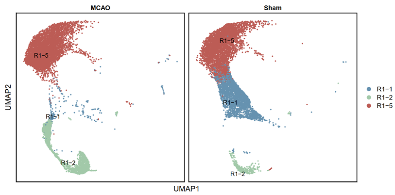
Save variable table as Round1.Rdata to continue. OR: Do not close R to ensure the subsequent programs can run.
Get the file GroupR1_2.h5ad and rename it to 2024.10.28_Group15-21.h5ad
Round 2
3 𝘿𝙞𝙨𝙩𝙞𝙣𝙜𝙪𝙞𝙨𝙝 𝙩𝙝𝙚 𝙨𝙩𝙖𝙜𝙚𝙨 𝙤𝙛 𝙛𝙚𝙧𝙧𝙤𝙥𝙩𝙤𝙨𝙞𝙨 𝙞𝙣 𝙘𝙚𝙡𝙡𝙨. 𝘿𝙪𝙚 𝙩𝙤 𝙨𝙝𝙖𝙧𝙚𝙙 𝙍𝙉𝘼 𝙥𝙖𝙩𝙝𝙬𝙖𝙮𝙨, 𝙢𝙖𝙣𝙮 𝙘𝙚𝙡𝙡𝙨 𝙪𝙣𝙙𝙚𝙧𝙜𝙤𝙞𝙣𝙜 𝙖𝙥𝙤𝙥𝙩𝙤𝙨𝙞𝙨 𝙖𝙧𝙚 𝙢𝙞𝙭𝙚𝙙 𝙞𝙣.
Start
3.1 𝐒𝐭𝐞𝐩 𝟏: 𝐀𝐜𝐭𝐢𝐯𝐚𝐭𝐞 𝐮𝐬𝐢𝐧𝐠 𝐭𝐡𝐞 𝐩𝐫𝐨𝐱𝐢𝐦𝐢𝐭𝐲 𝐦𝐞𝐭𝐡𝐨𝐝. (Python)
Import 2024.10.28_Group15-21.h5ad into [LittleSnowFox's Anaconda installation directory]\database\Tracing_sample\Nerveferroptosis_remove_R1_3_4\data\2024.10.28_Group15-21.h5ad.
import numpy as np
import os
import LittleSnowFox as kl
#import matlab.engine
#eng = matlab.engine.start_matlab()

print(kl.__version__)
# Initialization function to switch Kailin to the working directory.
# If it has been initialized before, running def kl_initialize(0) again
# will reject reinitialization to avoid recursion.
# Running def kl_initialize(1) will forcibly reinitialize.
kl.kl_initialize(0)

# Retrieve the root directory where Kailin works
parent_directory_origin = kl.kl_settings.parent_directory_origin
print(parent_directory_origin)

current_folder = kl.workcatalogue.choosemode_kl(parent_directory_origin,'Lineage',1)
print(current_folder)

# Select which sample to use
choosen_sample = "Nerveferroptosis_remove_R1_3_4"
# Select the .h5ad file
h5ad_filename = "2024.10.28_Group15-21.h5ad"
# Run the built-in example and obtain the sparse matrix
# Here, a non-example function needs to be included
current_folder_input = current_folder
orig_adata, loading_directory, distance_matrix = kl.preprocessing.kl_dense_matrix(
    choosen_sample,
    h5ad_filename,
    "draw",
    current_folder_input,
    1,
    13000,
    0.1,
    0.001,
    True
)
# orig_adata, loading_directory, distance_matrix_sparse = kl.preprocessing.kl_dense_matrix_sample(
#     choosen_sample,
#     h5ad_filename,
#     "draw",
#     current_folder_input
# )
# Run the built-in example and obtain the non-sparse matrix
# Here, a non-example function needs to be included
# current_folder_input = current_folder
# loading_directory, distance_matrix = kl.preprocessing.kl_dense_matrix(
#     choosen_sample,
#     h5ad_filename,
#     "draw",
#     current_folder_input
# )
print(loading_directory)
print(choosen_sample)


#需要区分dense和sparase
save_list = ["orig_adata.obsm['X_umap']"]

#将要计算的文件保存到/result
merged_csv,result_directory = kl.workcatalogue.kl_save(loading_directory,choosen_sample,distance_matrix,save_list,orig_adata)
3.2 𝐒𝐭𝐞𝐩 𝟐: 𝐔𝐬𝐞 𝐮𝐧𝐬𝐮𝐩𝐞𝐫𝐯𝐢𝐬𝐞𝐝 𝐥𝐞𝐚𝐫𝐧𝐢𝐧𝐠. (Matlab)
Afterward, execute the following file:
[LittleSnowFox's Anaconda installation directory]\database\Tracing_sample\Nerveferroptosis_remove_R1_3_4\main_v3_matlab_run_me.m
%% Load data and Split to compute
MM0 = load('./result/distance_matrix.mat');
MM0 = MM0.distance_matrix;

%% 读取要排序的对象
count_=readtable('./result/merged_data.csv');

%% 得到边界划分点
[p,splitlist] = binary_corr_sorting(MM0,20,500,5,5);%350:72 真实:68

%% 对划分点去重
[uniqueList, ~, ~] = unique(splitlist, 'stable');

%% 对相似度矩阵排序
MM=MM0(p,p);
split=[];

%% 重排count_result
count_result=count_(p,:);
split_simple=uniqueList;

%% 第一个起始位点置为1
split_simple(1)=1;
split_simple=[split_simple,length(MM0)];

%% 计算均值矩阵
[simple_matrix]=sample_computing(count_result,split_simple,MM,"mean");

%% 合并成小矩阵
ClusterReslut=cluster_map(split_simple,simple_matrix,0,0.0002,0);
count_result.Result = ClusterReslut;

%重排小矩阵
[cluster_map_matrix] = genetic_encoder( ...
    simple_matrix, ...
    60, ...% nPop = 50;  % 种群规模大小为30
    1, ...% nPc = 1; % 子代规模的比例0.8
    200, ...% maxIt = 200; % 最大迭代次数
    5 ...% cycletimes = 200; % 循环计算次数
    );


%重拍小矩阵方案2
% 创建行和列标签(示例)
%row_labels = cluster_map_label;
%column_labels = cluster_map_label;
% 使用 heatmap 函数并传递相应参数
h = heatmap(cluster_map_matrix);
%h.YDisplayLabels = row_labels; % 设置行标签
%h.XDisplayLabels = column_labels; % 设置列标签
h.ColorLimits = [0, 0.00007]

%----------------------------
figure(1)
h = heatmap(cluster_map_matrix);
h.ColorLimits = [0, 0.00007]


%writetable(count_result,"result/pseudotime_map.csv");

%% 临近法激活
corr_matrix = relevance_generate(0.000072,3,cluster_map_matrix);
heatmap(corr_matrix);

%% 编码
encode_result = encoder_corr_matrix(0.0000731,0.0000729,50,3,cluster_map_matrix);
figure(2)
hj = heatmap(encode_result);

%% 解码
figure(3)
[weighting_decode,decode_result] = decoder_corr_matrix(encode_result);
weighting_result = decode_result;
hk = heatmap(weighting_result);
hk.ColorLimits = [30, 35]

writetable(count_result,"result/pseudotime_map_R2.csv");
3.3 𝐒𝐭𝐞𝐩 𝟑: 𝐏𝐞𝐫𝐟𝐨𝐫𝐦 𝐨𝐦𝐢𝐜𝐬 𝐚𝐧𝐚𝐥𝐲𝐬𝐢𝐬. (R)
Open variable table as Round1.Rdata to continue. OR: You didn’t closed R.
3.3.1 Perform pseudo-time inference on groups 1, 2, and 5 (R)
#######################################Round 2##############################################
####3 Verify the ferroptosis ratio, distinguish between ferroptosis and apoptosis###########

####3.1 Step1: Activae....(Python)###########################

####3.2 Step 2: Use ... (Matlab)############################
##move the "pseudotime_map.csv" into"C:/GEOANALYSIS/GSE2324291w/output/Round2"

###3.3 Step 3: Perform omics analysis (R Studio)#########################
library(Seurat)
library(multtest)
library(dplyr)
library(ggplot2)
library(patchwork)
library(tidyverse)
library(UCell)
library(harmony)

setwd("C:/GEOANALYSIS/GSE2324291w")
##Load data
GR1_2=get(load(file = "./saves/Round2/GroupR1_2.Rdata"))
result_data <- read.csv("./output/Round2/pseudotime_map.csv", stringsAsFactors = FALSE)

##3.3.1 After analysis, import results from "pseudotime_map.csv" into metadata(R)##########
# First, create a new column 'Result2' and set it to NA, and Remove redundant metadata
GR1_2@meta.data$Result2 <- NA
columns_to_remove <- c("seurat_clusters", "RNA_snn_res.0.1", "Result", "CellGroupR1","CellGroupR1_label")
GR1_2@meta.data <- GR1_2@meta.data[, !colnames(GR1_2@meta.data) %in% columns_to_remove]

# Obtain the UMAP coordinates of GR1_2
umap_coords <- as.data.frame(Embeddings(GR1_2, reduction = "umap"))
colnames(umap_coords) <- c("Var1", "Var2")
umap_coords$cell_barcode <- rownames(umap_coords)
# Add an index column to the coordinates of result_data (row numbers correspond to cell order).
result_data$cell_index <- seq_len(nrow(result_data))
# Matching and merging using Var1 + Var2 as keys
umap_coords$key <- paste(round(umap_coords$Var1, 6), round(umap_coords$Var2, 6), sep = "_")
result_data$key <- paste(round(result_data$Var1, 6), round(result_data$Var2, 6), sep = "_")

merged <- merge(umap_coords, result_data[, c("key", "Result")], by = "key", all.x = TRUE)
rownames(merged) <- merged$cell_barcode

# Align according to GR1_2 cell order
matched_result <- merged[colnames(GR1_2), "Result"]

# Write metadata
GR1_2$Result2 <- matched_result

##3.3.2 Regrouping stressed neurons
# get the metadata
metadata <- GR1_2@meta.data
# Create new column 'CellGroupR2' based on 'Result' values
metadata$CellGroupR2 <- with(metadata,
                             ifelse(Result2 >= 1 & Result2 <= 4, "Group R2-1",
                                    ifelse(Result2 >= 5 & Result2 <= 7, "Group R2-2",
                                           ifelse(Result2 >= 8 & Result2 <= 12, "Group R2-3",
                                                  ifelse(Result2 >= 13 & Result2 <= 18, "Group R2-4", NA)))))
# Assign updated metadata back to the Seurat object
GR1_2@meta.data <- metadata
# Check results
head(GR1_2@meta.data)

##3.3.3 Begin classifying ferroptosis and apoptosis.
# Create a CellR2 object
CellR2 <- GR1_2
#Convert the matrix of GR1_2 to version 4
CellR2[["RNA"]] <- as(object = CellR2[["RNA"]], Class = "Assay")
#redo UMAP
CellR2 <- RunHarmony(CellR2, group.by.vars = "orig.ident")
CellR2 <- FindNeighbors(CellR2, reduction = "harmony", dims = 1:25) %>% FindClusters(resolution = 0.2)
CellR2 <- RunUMAP(CellR2, dims = 1:20,
                 spread = 0.5, n.neighbors = 100, min.dist = 0.5)

#(1) Define cell death-related genes
# Ferroptosis related genes
ferroptosis_driver <- c(
  "Acsl4",
  "Ptgs2",
  "Alox15",
  "Alox12",
  "Tfrc",
  "Lpcat3",
  "Ncoa4"
)

ferroptosis_suppressor <- c(
  "Gpx4",
  "Slc7a11",
  "Aifm2",
  "Nfe2l2",
  "Fth1",
  "Ftl1",
  "Gclc",
  "Gclm"
)

# Apoptosis-related genes
apoptosis_driver <- c(
  "Bax",
  "Bak1",
  "Bid",
  "Casp3",
  "Casp9",
  "Casp8",
  "Apaf1",
  "Cycs",
  "Trp53",
  "Fadd",
  "Bik",
  "Bad",
  "Bok",
  "Bmf",
  "Hrk",
  "Pmaip1",
  "Bcl2l11",
  "Bbc3"
)

apoptosis_suppressor <- c(
  "Bcl2",
  "Bcl2l1",
  "Mcl1",
  "Xiap",
  "Birc2",
  "Birc3",
  "Bcl2a1"
)

# Filtering existing genes
ferroptosis_driver <- ferroptosis_driver[ferroptosis_driver %in% rownames(CellR2)]
ferroptosis_suppressor <- ferroptosis_suppressor[ferroptosis_suppressor %in% rownames(CellR2)]
apoptosis_driver <- apoptosis_driver[apoptosis_driver %in% rownames(CellR2)]
apoptosis_suppressor <- apoptosis_suppressor[apoptosis_suppressor %in% rownames(CellR2)]

cat(sprintf("ferroptosis_driver genes: %d/%d detected\n", length(ferroptosis_driver), 7))
cat(sprintf("ferroptosis_suppressor genes: %d/%d detected\n", length(ferroptosis_suppressor), 8))
cat(sprintf("apoptosis_driver genes: %d/%d detected\n", length(apoptosis_driver), 18))
cat(sprintf("apoptosis_suppressor genes: %d/%d detected\n", length(apoptosis_suppressor), 7))

#(2) Calculate module scores
 # Calculate the ferroptosis_driver score
CellR2 <- AddModuleScore(
  CellR2,
  features = list(ferroptosis_driver),
  name = "Ferroptosis_Driver",
  ctrl = 50
)

# Calculate ferroptosis_suppressor score
CellR2 <- AddModuleScore(
  CellR2,
  features = list(ferroptosis_suppressor),
  name = "Ferroptosis_Suppressor",
  ctrl = 50
)

# Calculate apoptosis_driver score
CellR2 <- AddModuleScore(
  CellR2,
  features = list(apoptosis_driver),
  name = "Apoptosis_Driver",
  ctrl = 50
)

# Calculate Apoptosis_Suppressor score
CellR2 <- AddModuleScore(
  CellR2,
  features = list(apoptosis_suppressor),
  name = "Apoptosis_Suppressor",
  ctrl = 50
)

# (3) Calculate sum score
# Sum score = Driver + Inhibitor (reflecting the total activation level of the pathway).
CellR2$Ferroptosis_Sum <- CellR2$Ferroptosis_Driver1 + CellR2$Ferroptosis_Suppressor1
CellR2$Apoptosis_Sum <- CellR2$Apoptosis_Driver1 + CellR2$Apoptosis_Suppressor1

cat("✓ Sum score calculation completed\n")
cat(sprintf("  Ferroptosis_Sum range: [%.3f, %.3f]\n",
            min(CellR2$Ferroptosis_Sum), max(CellR2$Ferroptosis_Sum)))
cat(sprintf("  Apoptosis_Sum range: [%.3f, %.3f]\n",
            min(CellR2$Apoptosis_Sum), max(CellR2$Apoptosis_Sum)))

#(4) Calculate group characteristics
# Calculate the mean score and iron mortality advantage for each group
group_features <- CellR2@meta.data %>%
  group_by(CellGroupR2) %>%
  summarise(
    Avg_Ferro_Sum = mean(Ferroptosis_Sum),
    Avg_Apo_Sum = mean(Apoptosis_Sum),
    .groups = 'drop'
  ) %>%
  mutate(
    # Ferrocyte dominance = Ferrocyte Sum - Apoptosis Sum
    Ferro_Advantage = Avg_Ferro_Sum - Avg_Apo_Sum,
    # Ranked by dominance (1 = strongest apoptosis tendency, 5 = strongest ferroptosis tendency).
    Group_Rank = rank(Ferro_Advantage)
  ) %>%
  arrange(Group_Rank)

cat("\nFeatures of each CellGroup:\n")
print(group_features)

cat("\nAssign labels to groups based on ranking\n")
cat("Rank ≤ 2: Apoptosis-prone group\n")
cat("Rank = 3: Transition group\n")
cat("Rank ≥ 4: Ferrocyte-prone group\n\n")

# (5) Assign cell types
# Merge group features into cell metadata
meta <- CellR2@meta.data %>%
  left_join(group_features[, c("CellGroupR2", "Group_Rank", "Ferro_Advantage")],
            by = "CellGroupR2")

# Categorized based on group ranking and cell-specific score
meta$Death_Tendency <- with(meta, {
  case_when(
    # Rule 1: Groups with apoptosis propensity (rank ≤ 2)
    Group_Rank <= 2 & Apoptosis_Sum > Ferroptosis_Sum ~ "Apoptosis-prone",
    Group_Rank <= 2 ~ "Apoptosis-leaning",

    #  Rule 2: Groups with ferroptosis propensity (rank ≥ 4)
    Group_Rank >= 4 & Ferroptosis_Sum > Apoptosis_Sum ~ "Ferroptosis-prone",
    Group_Rank >= 4 ~ "Ferroptosis-leaning",

    #  Rule 3: Transitional group (rank = 3)
    TRUE ~ "Mixed"
  )
})

# Update metadata
CellR2@meta.data <- meta

cat("✓ Naming complete!\n\n")

# (6) Statistical results
# Overall Statistics
overall_summary <- CellR2@meta.data %>%
  group_by(Death_Tendency) %>%
  summarise(Count = n(), .groups = 'drop') %>%
  mutate(Proportion = round(Count / sum(Count) * 100, 1)) %>%
  arrange(desc(Count))

cat("[Overall Distribution]\n")
print(overall_summary)

# Stratified statistics by CellGroupR2
group_summary <- CellR2@meta.data %>%
  group_by(CellGroupR2, Death_Tendency) %>%
  summarise(Count = n(), .groups = 'drop') %>%
  group_by(CellGroupR2) %>%
  mutate(
    Total = sum(Count),
    Proportion = round(Count / Total * 100, 1)
  ) %>%
  arrange(CellGroupR2, desc(Proportion))

cat("\n[Stratified by CellGroup]\n")
print(group_summary)

# Intergroup differentiation
cat("\n[Intergroup Differentiation Examination]\n")
dominant_types <- group_summary %>%
  group_by(CellGroupR2) %>%
  slice_max(Proportion, n = 1) %>%
  pull(Death_Tendency)

ferro_groups <- unique(group_summary$CellGroupR2[grepl("Ferroptosis",
                                                       group_summary$Death_Tendency) &
                                                   group_summary$Proportion > 50])
apo_groups <- unique(group_summary$CellGroupR2[grepl("Apoptosis",
                                                     group_summary$Death_Tendency) &
                                                 group_summary$Proportion > 50])
mixed_groups <- unique(group_summary$CellGroupR2[group_summary$Death_Tendency == "Mixed" &
                                                   group_summary$Proportion > 50])

cat(sprintf("Ferropion-dominated group: %s\n", paste(ferro_groups, collapse = ", ")))
cat(sprintf("Apoptosis-dominated group: %s\n", paste(apo_groups, collapse = ", ")))
cat(sprintf("Mixed group: %s\n", paste(mixed_groups, collapse = ", ")))

if (length(ferro_groups) >= 1 && length(apo_groups) >= 1) {
  cat("\n✓✓✓  uccessfully achieved intergroup differentiation!\n")
} else {
  cat("\n⚠ Differentiation effect is not ideal\n")
}

#(8) Cell nomenclature
# get the metadata
metadata <- CellR2@meta.data
# Create new column 'CellGroupR2' based on 'Result' values
metadata$CellNameR2 <- with(metadata,
                            ifelse(CellGroupR2 == "Group R2-1", "Mixed",
                                   ifelse(CellGroupR2 == "Group R2-2", "Apoptosis",
                                          ifelse(CellGroupR2 == "Group R2-3", "Apoptosis",
                                                 ifelse(CellGroupR2 == "Group R2-4", "Ferroptosis", NA)))))

# Assign updated metadata back to the Seurat object
CellR2@meta.data <- metadata
# Check results
head(CellR2@meta.data)

#Add CellNameR2 to the state_summary table.
# === Add CellNameR2 to group_summary ===
group_summary <- group_summary %>%
  mutate(CellNameR2 = recode(CellGroupR2,
                             "Group R2-1" = "Mixed",
                             "Group R2-2" = "Apoptosis",
                             "Group R2-3" = "Apoptosis",
                             "Group R2-4" = "Ferroptosis"))

# Check
cat("group_summary with CellNameR2:\n")
print(head(group_summary))

# === Add CellNameR2 to overall_summary ===
# Note: overall_summary typically doesn't have CellGroupR2
# If it has, use the same approach:
if ("CellGroupR2" %in% colnames(overall_summary)) {
  overall_summary <- overall_summary %>%
    mutate(CellNameR2 = recode(CellGroupR2,
                               "Group R2-1" = "Mixed",
                               "Group R2-2" = "Apoptosis",
                               "Group R2-3" = "Apoptosis",
                               "Group R2-4" = "Ferroptosis"))

  cat("\noverall_summary with CellNameR2:\n")
  print(head(overall_summary))
}

# === Add CellNameR2 to group_features ===
group_features <- group_features %>%
  mutate(CellNameR2 = recode(CellGroupR2,
                             "Group R2-1" = "Mixed",
                             "Group R2-2" = "Apoptosis",
                             "Group R2-3" = "Apoptosis",
                             "Group R2-4" = "Ferroptosis"))

# Check
cat("\ngroup_features with CellNameR2:\n")
print(group_features)

#(8) Save the results
# Create output directory
if (!dir.exists("./output/Round2/DeathType_Results")) {
  dir.create("./output/Round2/DeathType_Results", recursive = TRUE)
}
if (!dir.exists("./figures/Round2/DeathType_Results")) {
  dir.create("./figures/Round2/DeathType_Results", recursive = TRUE)
}

# Save Seurat obj
saveRDS(CellR2, "./saves/Round2/CellR2_DeathType.rds")
save(CellR2, file = "./saves/Round2/CellR2_DeathType.Rdata")

# Save tables
write.csv(overall_summary,
          "./output/Round2/DeathType_Results/overall_summary.csv",
          row.names = FALSE)

write.csv(group_summary,
          "./output/Round2/DeathType_Results/group_summary.csv",
          row.names = FALSE)

write.csv(group_features,
          "./output/Round2/DeathType_Results/group_features.csv",
          row.names = FALSE)

cat("✓ Data file saved successfully\n\n")


# (9) Visualization
# === Color Settings ===
death_colors <- c(
  "Ferroptosis-prone" = "#DC0000",
  "Ferroptosis-leaning" = "#F39B7F",
  "Mixed" = "#00A087",
  "Apoptosis-leaning" = "#91D1C2",
  "Apoptosis-prone" = "#3C5488"
)

cellname_colors <- c(
  "Ferroptosis" = "#bd5c56",
  "Apoptosis" = "#6693b1",
  "Mixed" = "#a3caa9"
)

# === Extract UMAP Coordinates ===
cat("Extracting UMAP coordinates...\n")

umap_data <- as.data.frame(Embeddings(CellR2, reduction = "umap"))
colnames(umap_data) <- c("UMAP_1", "UMAP_2")

# Add metadata
umap_data$Death_Tendency <- CellR2$Death_Tendency
umap_data$CellNameR2 <- CellR2$CellNameR2
umap_data$CellGroupR2 <- CellR2$CellGroupR2
umap_data$Group <- CellR2$Group
umap_data$seurat_clusters <- CellR2$seurat_clusters
umap_data$Ferroptosis_Sum <- CellR2$Ferroptosis_Sum
umap_data$Apoptosis_Sum <- CellR2$Apoptosis_Sum

cat(sprintf("UMAP data prepared: %d cells\n", nrow(umap_data)))

# === Create Summary Tables for CellNameR2 ===
cat("\nCreating summary tables for CellNameR2...\n")

# Overall summary by CellNameR2
cellname_overall <- CellR2@meta.data %>%
  group_by(CellNameR2) %>%
  summarise(Count = n(), .groups = 'drop') %>%
  mutate(Proportion = round(Count / sum(Count) * 100, 1)) %>%
  arrange(desc(Count))

cat("CellNameR2 overall distribution:\n")
print(cellname_overall)

# Summary by CellGroupR2 and CellNameR2
cellname_by_group <- CellR2@meta.data %>%
  group_by(CellGroupR2, CellNameR2) %>%
  summarise(Count = n(), .groups = 'drop') %>%
  group_by(CellGroupR2) %>%
  mutate(
    Total = sum(Count),
    Proportion = round(Count / Total * 100, 1)
  ) %>%
  arrange(CellGroupR2, desc(Proportion))

cat("\nCellNameR2 by CellGroupR2:\n")
print(cellname_by_group)

# Summary by Group (MCAO/Sham) and CellNameR2
cellname_by_mcao <- CellR2@meta.data %>%
  group_by(Group, CellGroupR2, CellNameR2) %>%
  summarise(Count = n(), .groups = 'drop') %>%
  group_by(Group, CellGroupR2) %>%
  mutate(
    Total = sum(Count),
    Proportion = round(Count / Total * 100, 1)
  )

# Create summary: CellNameR2 as x-axis, Death_Tendency as fill
cellname_death_summary <- CellR2@meta.data %>%
  group_by(CellNameR2, Death_Tendency) %>%
  summarise(Count = n(), .groups = 'drop') %>%
  group_by(CellNameR2) %>%
  mutate(
    Total = sum(Count),
    Proportion = round(Count / Total * 100, 1)
  ) %>%
  arrange(CellNameR2, desc(Proportion))

# === Create Output Directories ===
dir.create("./figures/Round2/DeathType_Results", showWarnings = FALSE, recursive = TRUE)
dir.create("./figures/Round2/CellNameR2_Results", showWarnings = FALSE, recursive = TRUE)

# ============================================
# Section A: Death_Tendency Figures
# ============================================
cat("\n========================================\n")
cat("Section A: Death_Tendency Visualizations\n")
cat("========================================\n\n")

# === A1: Stacked Bar Chart by Death_Tendency ===
cat("Generating A1: Bar chart by Death_Tendency...\n")

pA1_barplot <- ggplot(group_summary,
                      aes(x = CellGroupR2, y = Proportion, fill = Death_Tendency)) +
  geom_bar(stat = "identity", width = 0.7) +
  geom_text(aes(label = sprintf("%.1f%%", Proportion)),
            position = position_stack(vjust = 0.5),
            size = 3.5, color = "white", fontface = "bold") +
  scale_fill_manual(values = death_colors) +
  theme_classic(base_size = 14) +
  labs(title = "Cell Death Tendency Distribution by Cell Group",
       x = "Cell Group", y = "Percentage (%)", fill = "Death Tendency") +
  theme(plot.title = element_text(hjust = 0.5, face = "bold", size = 16),
        axis.text.x = element_text(angle = 45, hjust = 1, size = 12),
        legend.position = "right")

ggsave("./figures/Round2/DeathType_Results/A1_barplot_death_tendency.pdf",
       pA1_barplot, width = 8, height = 6)

# === A2: UMAP by Death_Tendency ===
cat("Generating A2: UMAP by Death_Tendency...\n")

pA2_umap <- ggplot(umap_data, aes(x = UMAP_1, y = UMAP_2, color = Death_Tendency)) +
  geom_point(size = 1, alpha = 0.8) +
  scale_color_manual(values = death_colors, name = "Death Tendency") +
  theme_classic(base_size = 14) +
  ggtitle("Cell Death Tendency in UMAP Space") +
  labs(x = "UMAP1", y = "UMAP2") +
  theme(plot.title = element_text(hjust = 0.5, face = "bold", size = 16),
        legend.position = "right",
        panel.border = element_rect(fill = NA, color = "black", size = 1),
        axis.text = element_blank(), axis.ticks = element_blank())

ggsave("./figures/Round2/DeathType_Results/A2_umap_death_tendency.pdf",
       pA2_umap, width = 7.5, height = 5.5)

# ============================================
# Section B: CellNameR2 Figures
# ============================================
cat("\n========================================\n")
cat("Section B: CellNameR2 Visualizations\n")
cat("========================================\n\n")

# === B1: Stacked Bar Chart by CellNameR2 ===
cat("Generating B1: Bar chart by CellNameR2...\n")

pB1_barplot <- ggplot(cellname_death_summary,
                      aes(x = CellNameR2, y = Proportion, fill = Death_Tendency)) +
  geom_bar(stat = "identity", width = 0.7) +
  geom_text(aes(label = sprintf("%.1f%%", Proportion)),
            position = position_stack(vjust = 0.5),
            size = 3.5, color = "white", fontface = "bold") +
  scale_fill_manual(values = death_colors) +
  theme_classic(base_size = 14) +
  labs(title = "Death Tendency Distribution by Cell Type",
       x = "Cell Type", y = "Percentage (%)", fill = "Death Tendency") +
  theme(plot.title = element_text(hjust = 0.5, face = "bold", size = 16),
        axis.text.x = element_text(angle = 0, hjust = 0.5, size = 12),
        axis.text.y = element_text(size = 12),
        legend.position = "right",
        legend.title = element_text(size = 12),
        legend.text = element_text(size = 11))

ggsave("./figures/Round2/CellNameR2_Results/B1_barplot_cellname_by_death.pdf",
       pB1_barplot, width = 7, height = 6)

# === B2: UMAP by CellNameR2 ===
cat("Generating B2: UMAP by CellNameR2...\n")

pB2_umap <- ggplot(umap_data, aes(x = UMAP_1, y = UMAP_2, color = CellNameR2)) +
  geom_point(size = 1, alpha = 0.8) +
  scale_color_manual(values = cellname_colors, name = "Cell Type") +
  theme_classic(base_size = 14) +
  ggtitle("Cell Types in UMAP Space") +
  labs(x = "UMAP1", y = "UMAP2") +
  theme(plot.title = element_text(hjust = 0.5, face = "bold", size = 16),
        legend.position = "right",
        panel.border = element_rect(fill = NA, color = "black", size = 1),
        axis.text = element_blank(), axis.ticks = element_blank())

ggsave("./figures/Round2/CellNameR2_Results/B2_umap_cellname.pdf",
       pB2_umap, width = 7.5, height = 5.5)

# ============================================
# Section C: Additional Reference Figures
# ============================================
cat("\n========================================\n")
cat("Section C: Additional Figures\n")
cat("========================================\n\n")

# === C1: UMAP by Seurat Clusters ===
cat("Generating C1: UMAP by seurat_clusters...\n")

pC1_clusters <- ggplot(umap_data, aes(x = UMAP_1, y = UMAP_2, color = seurat_clusters)) +
  geom_point(size = 1, alpha = 0.8) +
  theme_classic(base_size = 14) +
  ggtitle("Seurat Clusters in UMAP Space") +
  labs(x = "UMAP1", y = "UMAP2", color = "Cluster") +
  theme(plot.title = element_text(hjust = 0.5, face = "bold", size = 16),
        legend.position = "right",
        panel.border = element_rect(fill = NA, color = "black", size = 1),
        axis.text = element_blank(), axis.ticks = element_blank())

ggsave("./figures/Round2/DeathType_Results/C1_umap_clusters.pdf",
       pC1_clusters, width = 6.5, height = 5.5)

# === C2: UMAP with All Cells in Gray (Reference Map) ===
cat("Generating C2: UMAP reference map (all cells gray)...\n")

pC2_gray <- ggplot(umap_data, aes(x = UMAP_1, y = UMAP_2)) +
  geom_point(size = 1, alpha = 0.6, color = "gray70") +
  theme_classic(base_size = 14) +
  ggtitle("UMAP - All Cells") +
  labs(x = "UMAP1", y = "UMAP2") +
  theme(
    plot.title = element_text(hjust = 0.5, face = "bold", size = 16),
    panel.border = element_rect(fill = NA, color = "black", size = 1),
    axis.text = element_blank(),
    axis.ticks = element_blank()
  )

ggsave("./figures/Round2/DeathType_Results/C2_umap_gray_reference.pdf",
       pC2_gray, width = 5.5, height = 5.5)

cat("✓ Additional figures complete\n")

###3.4 GSVA of ferroptosis and apoptosis in cells
setwd("C:/GEOANALYSIS/GSE2324291w")

library(Seurat)
library(GSVA)
library(msigdbr)
library(limma)
library(dplyr)
library(ggplot2)
library(openxlsx)
library(BiocParallel)

cat("============================================\n")
cat("GSVA Analysis: Ferroptosis vs Apoptosis\n")
cat("WITH MULTI-THREADING\n")
cat("============================================\n\n")

# ============================================
# Step 0: Setup Parallel Computing
# ============================================
cat("【Step 0】Setting up parallel computing...\n")

# Detect available cores
n_cores <- parallel::detectCores()
cat(sprintf("Total CPU cores detected: %d\n", n_cores))

# Use maximum 4 cores (recommended for memory efficiency)
n_workers <- min(14, n_cores - 10)  # Leave 1 core for system
cat(sprintf("Using %d cores for parallel computing\n", n_workers))

# Setup parallel backend
if (.Platform$OS.type == "windows") {
  # Windows: use SnowParam
  BPPARAM <- SnowParam(workers = n_workers, type = "SOCK", progressbar = TRUE)
  cat("Parallel backend: SnowParam (Windows)\n")
} else {
  # Unix/Mac: use MulticoreParam
  BPPARAM <- MulticoreParam(workers = n_workers, progressbar = TRUE)
  cat("Parallel backend: MulticoreParam (Unix/Mac)\n")
}

cat(sprintf("✓ Parallel computing configured: %d workers\n\n", n_workers))

# ============================================
# Step 1: Load Data
# ============================================
cat("【Step 1】Loading CellR2 object...\n")

# Load the Seurat object
CellR2 <- readRDS("./saves/Round2/CellR2_DeathType.rds")
# Or use: load("./saves/Round2/CellR2_DeathType.Rdata")

cat(sprintf("Total cells: %d\n", ncol(CellR2)))
cat("CellNameR2 distribution:\n")
print(table(CellR2$CellNameR2))

# ============================================
# Step 2: Define Gene Set Configurations
# ============================================
cat("\n【Step 2】Defining gene set configurations...\n")

gene_set_configs <- list(
  list(name = "HALLMARK",     category = "H",  subcategory = NULL),
  list(name = "GO_BP",        category = "C5", subcategory = "GO:BP"),
  list(name = "GO_CC",        category = "C5", subcategory = "GO:CC"),
  list(name = "GO_MF",        category = "C5", subcategory = "GO:MF"),
  list(name = "REACTOME",     category = "C2", subcategory = "CP:REACTOME"),
  list(name = "WIKIPATHWAYS", category = "C2", subcategory = "CP:WIKIPATHWAYS"),
  list(name = "BIOCARTA",     category = "C2", subcategory = "CP:BIOCARTA")
)

cat(sprintf("Total gene set collections: %d\n", length(gene_set_configs)))

# ============================================
# Step 3: Download All Gene Sets
# ============================================
cat("\n【Step 3】Downloading gene sets from MSigDB...\n")

all_gene_sets <- list()

for (config in gene_set_configs) {
  cat(sprintf("\nDownloading %s...\n", config$name))

  tryCatch({
    # Download from MSigDB (Homo sapiens)
    msigdb_data <- msigdbr(
      species = "Homo sapiens",
      category = config$category,
      subcategory = config$subcategory
    )

    if (nrow(msigdb_data) == 0) {
      cat(sprintf("  ⚠️ No gene sets found for %s\n", config$name))
      next
    }

    # Convert to list format
    gene_sets <- msigdb_data %>%
      split(x = .$gene_symbol, f = .$gs_name)

    # Store
    all_gene_sets[[config$name]] <- gene_sets

    cat(sprintf("  ✓ Downloaded %d gene sets\n", length(gene_sets)))

    # Clean up
    rm(msigdb_data, gene_sets)
    gc()

  }, error = function(e) {
    cat(sprintf("  ✗ Failed: %s\n", e$message))
  })
}

cat(sprintf("\n✓ Total collections downloaded: %d\n", length(all_gene_sets)))

# ============================================
# Step 4-5: Filter Cells and Prepare Matrix (CORRECTED)
# ============================================
cat("\n【Step 4-5】Filtering cells and preparing expression matrix...\n")

# Use INDICES to select cells (not cell names)
cat("Identifying cell indices by CellNameR2...\n")
ferro_idx <- which(CellR2$CellNameR2 == "Ferroptosis")
apo_idx <- which(CellR2$CellNameR2 == "Apoptosis")

cat(sprintf("Ferroptosis cells: %d\n", length(ferro_idx)))
cat(sprintf("Apoptosis cells: %d\n", length(apo_idx)))
cat(sprintf("Total cells: %d\n", length(ferro_idx) + length(apo_idx)))

# Combine indices
cells_idx <- c(ferro_idx, apo_idx)

# Extract expression matrix using INDICES
cat("\nExtracting expression matrix...\n")
expr_matrix <- GetAssayData(CellR2, slot = "data")[, cells_idx]

cat(sprintf("Expression matrix: %d genes × %d cells\n",
            nrow(expr_matrix), ncol(expr_matrix)))

# Get actual cell barcodes from the matrix
cell_barcodes <- colnames(expr_matrix)

# Create group vector with barcode names
cat("Creating group vector...\n")
group_vec <- CellR2$CellNameR2[cells_idx]
names(group_vec) <- cell_barcodes

cat("Group distribution:\n")
print(table(group_vec))

# Convert gene names to human format
cat("\nConverting gene names to human (uppercase)...\n")
rownames(expr_matrix) <- toupper(rownames(expr_matrix))

if ("TRFC" %in% rownames(expr_matrix)) {
  rownames(expr_matrix)[rownames(expr_matrix) == "TRFC"] <- "TF"
}

# Filter genes
cat("Filtering genes (>= 1% cells)...\n")
min_cells <- ceiling(ncol(expr_matrix) * 0.01)
gene_counts <- Matrix::rowSums(expr_matrix > 0)
genes_to_keep <- gene_counts >= min_cells

cat(sprintf("  Original: %d genes\n", nrow(expr_matrix)))
cat(sprintf("  Kept: %d genes\n", sum(genes_to_keep)))

expr_matrix_filtered <- expr_matrix[genes_to_keep, ]

cat(sprintf("\n✓ Final matrix: %d genes × %d cells\n",
            nrow(expr_matrix_filtered), ncol(expr_matrix_filtered)))

# Verification
cat("\n【Verification】\n")
cat(sprintf("Matrix cells: %d\n", ncol(expr_matrix_filtered)))
cat(sprintf("Group vector: %d\n", length(group_vec)))
cat(sprintf("Match: %s\n", all(colnames(expr_matrix_filtered) == names(group_vec))))

cat("\nFinal distribution:\n")
print(table(group_vec))

# Clean up
rm(expr_matrix)
gc()

# ============================================
# Step 6: Create Output Directories
# ============================================
cat("\n【Step 6】Creating output directories...\n")

output_dir <- "./output/Round2/GSVA_Ferroptosis_vs_Apoptosis"
figure_dir <- "./figures/Round2/GSVA_Ferroptosis_vs_Apoptosis"

dir.create(output_dir, showWarnings = FALSE, recursive = TRUE)
dir.create(figure_dir, showWarnings = FALSE, recursive = TRUE)

cat(sprintf("Output: %s\n", output_dir))
cat(sprintf("Figures: %s\n", figure_dir))

# ============================================
# Step 7: Define GSVA Function
# ============================================
cat("\n【Step 7】Defining GSVA analysis function...\n")

run_gsva_limma <- function(expr_mat, group_vec, ref_level, contrast_level,
                           gene_sets, set_name, BPPARAM) {

  cat(sprintf("\n--- Analyzing %s ---\n", set_name))
  cat(sprintf("Gene sets: %d\n", length(gene_sets)))
  cat(sprintf("Parallel workers: %d\n", bpnworkers(BPPARAM)))

  # Convert to dense matrix
  cat("Converting to dense matrix...\n")
  expr_mat_dense <- as.matrix(expr_mat)

  # Run GSVA
  cat("Running GSVA with multi-threading...\n")
  start_time <- Sys.time()

  gsva_result <- gsva(
    expr = expr_mat_dense,
    gset.idx.list = gene_sets,
    method = "gsva",
    kcdf = "Poisson",
    verbose = TRUE,
    BPPARAM = BPPARAM
  )

  elapsed <- difftime(Sys.time(), start_time, units = "mins")
  cat(sprintf("✓ GSVA completed in %.2f minutes\n", as.numeric(elapsed)))

  rm(expr_mat_dense)
  gc()

  # limma analysis
  cat("Running limma...\n")
  group_factor <- factor(group_vec, levels = c(ref_level, contrast_level))
  design <- model.matrix(~ group_factor)
  colnames(design) <- c("Intercept", paste0(contrast_level, "_vs_", ref_level))

  fit <- eBayes(lmFit(gsva_result, design))

  results <- topTable(
    fit,
    coef = paste0(contrast_level, "_vs_", ref_level),
    number = Inf,
    adjust.method = "BH"
  )

  results$Pathway <- rownames(results)
  results <- results[, c("Pathway", "logFC", "AveExpr", "t", "P.Value", "adj.P.Val", "B")]

  n_sig <- sum(results$adj.P.Val < 0.05)
  cat(sprintf("✓ Significant: %d / %d\n", n_sig, nrow(results)))

  return(results)
}

cat("✓ Function defined\n")

# ============================================
# Step 8: Run GSVA for All Gene Sets
# ============================================
cat("\n【Step 8】Running GSVA for all gene sets...\n")
cat(sprintf("Using %d parallel workers per gene set\n\n", n_workers))

wb <- createWorkbook()
all_results <- list()

total_start <- Sys.time()

for (set_name in names(all_gene_sets)) {

  cat(sprintf("\n========================================\n"))
  cat(sprintf("Processing: %s\n", set_name))
  cat(sprintf("========================================\n"))

  results <- run_gsva_limma(
    expr_mat = expr_matrix_filtered,
    group_vec = group_vec,
    ref_level = "Apoptosis",
    contrast_level = "Ferroptosis",
    gene_sets = all_gene_sets[[set_name]],
    set_name = set_name,
    BPPARAM = BPPARAM
  )

  all_results[[set_name]] <- results

  # Save to Excel
  addWorksheet(wb, set_name)
  writeData(wb, set_name, results)

  # Save CSV
  csv_file <- file.path(output_dir, paste0("GSVA_", set_name, ".csv"))
  write.csv(results, csv_file, row.names = FALSE)
  cat(sprintf("✓ Saved: %s\n", basename(csv_file)))

  gc()
}

total_elapsed <- difftime(Sys.time(), total_start, units = "mins")
cat(sprintf("\n✓ All completed in %.2f minutes\n", as.numeric(total_elapsed)))

# Save Excel
excel_file <- file.path(output_dir, "GSVA_Ferroptosis_vs_Apoptosis_All_Results.xlsx")
saveWorkbook(wb, excel_file, overwrite = TRUE)
cat(sprintf("✓ Excel saved: %s\n", basename(excel_file)))

# ============================================
# Step 9: Create Summary Statistics
# ============================================
cat("\n【Step 9】Creating summary statistics...\n")

summary_stats <- data.frame(
  Gene_Set = names(all_results),
  Total_Pathways = sapply(all_results, nrow),
  Significant_FDR005 = sapply(all_results, function(x) sum(x$adj.P.Val < 0.05)),
  Significant_FDR01 = sapply(all_results, function(x) sum(x$adj.P.Val < 0.01)),
  Upregulated_in_Ferro = sapply(all_results, function(x) sum(x$adj.P.Val < 0.05 & x$logFC > 0)),
  Downregulated_in_Ferro = sapply(all_results, function(x) sum(x$adj.P.Val < 0.05 & x$logFC < 0))
)

cat("\nSummary statistics:\n")
print(summary_stats)

# Save summary
summary_file <- file.path(output_dir, "GSVA_Summary_Statistics.csv")
write.csv(summary_stats, summary_file, row.names = FALSE)
cat(sprintf("✓ Summary saved: %s\n", basename(summary_file)))


##3.5 Create GSVA plot for Round2
library(ggplot2)
library(dplyr)
library(openxlsx)
library(ggrepel)
library(stringr)

# ────────────────────────────────────────────
# Set paths (modify according to your actual paths)
# ────────────────────────────────────────────
excel_file <- "./output/Round2/GSVA_Ferroptosis_vs_Apoptosis/GSVA_Ferroptosis_vs_Apoptosis_All_Results.xlsx"
output_dir <- "./output/Round2/GSVA_Ferroptosis_vs_Apoptosis"
figure_dir <- "./figures/Round2/GSVA_Ferroptosis_vs_Apoptosis"

# Ensure figure directory exists
dir.create(figure_dir, showWarnings = FALSE, recursive = TRUE)

# Custom figures go directly to figure_dir
custom_fig_dir <- figure_dir

# ────────────────────────────────────────────
# User-defined pathways to highlight (same as Round1)
# ────────────────────────────────────────────
user_specified_pathways <- c(
  "GOBP_MULTICELLULAR_ORGANISMAL_LEVEL_IRON_ION_HOMEOSTASIS",
  "GOBP_TRANSFERRIN_TRANSPORT",
  "GOBP_NEGATIVE_REGULATION_OF_APOPTOTIC_SIGNALING_PATHWAY",
  "GOBP_NEGATIVE_REGULATION_OF_FERROPTOSIS",
  "GOBP_FERROPTOSIS",
  "GOBP_NEGATIVE_REGULATION_OF_INTRINSIC_APOPTOTIC_SIGNALING_PATHWAY",
  "GOBP_REGULATION_OF_IRON_ION_TRANSPORT",
  "GOBP_NEGATIVE_REGULATION_OF_OXIDATIVE_STRESS_INDUCED_INTRINSIC_APOPTOTIC_SIGNALING_PATHWAY",
  "GOBP_CELLULAR_RESPONSE_TO_IRON_ION",
  "GOBP_NEGATIVE_REGULATION_OF_MITOCHONDRIAL_OUTER_MEMBRANE_PERMEABILIZATION_INVOLVED_IN_APOPTOTIC_SIGNALING_PATHWAY",
  "GOBP_INTRACELLULAR_IRON_ION_HOMEOSTASIS",
  "GOBP_NEGATIVE_REGULATION_OF_INTRINSIC_APOPTOTIC_SIGNALING_PATHWAY_IN_RESPONSE_TO_DNA_DAMAGE",
  "GOBP_IRON_ION_TRANSPORT",
  "GOBP_MITOCHONDRIAL_FRAGMENTATION_INVOLVED_IN_APOPTOTIC_PROCESS",
  "GOBP_REGULATION_OF_MOTOR_NEURON_APOPTOTIC_PROCESS",
  "GOBP_IRON_ION_IMPORT_ACROSS_PLASMA_MEMBRANE",
  "GOBP_IRON_IMPORT_INTO_CELL",
  "GOBP_REGULATION_OF_IRON_ION_TRANSMEMBRANE_TRANSPORT",
  "GOBP_RESPONSE_TO_IRON_ION",
  "GOBP_REGULATION_OF_NEURON_APOPTOTIC_PROCESS",
  "GOBP_MOTOR_NEURON_APOPTOTIC_PROCESS",
  "GOBP_RESPONSE_TO_IRON_II_ION",
  "GOBP_NEURON_APOPTOTIC_PROCESS"
)
# ────────────────────────────────────────────
# Function: Custom Barplot for a single gene set
# ────────────────────────────────────────────
plot_custom_barplot <- function(result_df, gene_set_name, pathways_to_show, top_n = 30) {

  if (is.null(result_df) || nrow(result_df) == 0) {
    cat(sprintf("No results for %s. Skipping barplot.\n", gene_set_name))
    return(NULL)
  }

  # More relaxed matching: remove common prefixes for better filtering
  pattern <- paste0("^(", paste(pathways_to_show, collapse = "|"), ")$")
  filtered <- result_df %>%
    mutate(
      # Clean pathway name: remove prefixes (GOBP_, GOCC_, etc.) and replace underscores with spaces
      Pathway_clean = gsub("^(GO|GOBP|GOMF|GOCC|REACTOME)_", "", Pathway),
      Pathway_clean = gsub("_", " ", Pathway_clean)
    ) %>%
    filter(grepl(pattern, Pathway, ignore.case = TRUE) |
             grepl(pattern, Pathway_clean, ignore.case = TRUE)) %>%
    arrange(desc(abs(logFC))) %>%
    head(top_n)

  if (nrow(filtered) == 0) {
    cat(sprintf("No matching pathways found in %s.\n", gene_set_name))
    return(NULL)
  }

  cat(sprintf("Found %d matching pathways in %s:\n", nrow(filtered), gene_set_name))
  print(head(filtered$Pathway, 5))  # Debug: show first 5 matched pathways

  # Create short, clean label: remove prefix, replace underscore, and auto-wrap
  filtered$Pathway_short <- gsub("^(GO|GOBP|GOMF|GOCC|REACTOME)_", "", filtered$Pathway)
  filtered$Pathway_short <- gsub("_", " ", filtered$Pathway_short)
  filtered$Pathway_short <- str_wrap(filtered$Pathway_short, width = 35)  # Auto line break: 35 chars per line

  filtered$Direction <- ifelse(filtered$logFC > 0, "Up in Ferroptosis", "Down in Ferroptosis")

  p <- ggplot(filtered,
              aes(x = reorder(Pathway_short, logFC),
                  y = logFC,
                  fill = Direction)) +
    geom_bar(stat = "identity", width = 0.7) +
    coord_flip() +
    scale_fill_manual(values = c("Up in Ferroptosis" = "#E64B35", "Down in Ferroptosis" = "#4DBBD5")) +
    geom_hline(yintercept = 0, linetype = "solid", color = "black") +
    theme_classic(base_size = 10) +
    labs(title = paste("Custom Pathways:", gene_set_name),
         subtitle = paste("Shown:", nrow(filtered), "pathways | Ferroptosis vs Apoptosis"),
         x = "Pathway", y = "logFC (Ferroptosis - Apoptosis)", fill = NULL) +
    theme(
      plot.title = element_text(hjust = 0.5, face = "bold", size = 13),
      plot.subtitle = element_text(hjust = 0.5, size = 10),
      axis.text.x = element_text(size = 9),
      axis.text.y = element_text(size = 9, lineheight = 0.8),  # Helps readability of wrapped text
      axis.title = element_text(size = 11),
      legend.text = element_text(size = 9),
      legend.title = element_text(size = 10)
    )

  # Save (dynamic height based on number of pathways)
  fname <- paste0("Custom_Barplot_", gene_set_name, "_Round2.pdf")
  ggsave(file.path(custom_fig_dir, fname), p, width = 14, height = max(8, nrow(filtered)*0.5))

  cat(sprintf("✓ Barplot saved: %s\n", fname))
  return(p)
}

# ────────────────────────────────────────────
# Function: Custom Volcano plot for a single gene set
# ────────────────────────────────────────────
plot_custom_volcano <- function(result_df, gene_set_name, pathways_to_label, pval_thresh = 0.05, logfc_thresh = 0) {

  if (is.null(result_df) || nrow(result_df) == 0) return(NULL)

  df <- result_df %>%
    mutate(
      Significance = case_when(
        adj.P.Val < pval_thresh & abs(logFC) > logfc_thresh & logFC > 0 ~ "Up",
        adj.P.Val < pval_thresh & abs(logFC) > logfc_thresh & logFC < 0 ~ "Down",
        TRUE ~ "NS"
      ),
      # Clean pathway name: remove prefixes and replace underscores
      Pathway_clean = gsub("^(GO|GOBP|GOMF|GOCC|REACTOME)_", "", Pathway),
      Pathway_clean = gsub("_", " ", Pathway_clean)
    )

  # More relaxed matching for labeling
  pattern <- paste0("^(", paste(pathways_to_label, collapse = "|"), ")$")
  df$Label <- ""
  to_label <- df %>% filter(grepl(pattern, Pathway, ignore.case = TRUE) |
                              grepl(pattern, Pathway_clean, ignore.case = TRUE))

  if (nrow(to_label) == 0) {
    cat(sprintf("Warning: No pathways matched for labeling in %s.\n", gene_set_name))
  } else {
    cat(sprintf("Labeling %d pathways in %s:\n", nrow(to_label), gene_set_name))
    print(head(to_label$Pathway, 5))
  }

  # Set label: cleaned name + auto-wrap
  df$Label[match(to_label$Pathway, df$Pathway)] <- str_wrap(to_label$Pathway_clean, width = 25)

  p <- ggplot(df, aes(x = logFC, y = -log10(P.Value), color = Significance)) +
    geom_point(alpha = 0.7, size = 2.8) +
    geom_vline(xintercept = 0, linetype = "dashed", color = "gray50") +
    geom_hline(yintercept = -log10(pval_thresh), linetype = "dashed", color = "gray50") +
    scale_color_manual(values = c("Up" = "#E64B35", "Down" = "#4DBBD5", "NS" = "gray80")) +
    geom_text_repel(aes(label = Label),
                    size = 3.0,
                    max.overlaps = Inf,
                    box.padding = 1.0,
                    point.padding = 0.6,
                    segment.color = "grey50",
                    segment.size = 0.3,
                    min.segment.length = 0,
                    lineheight = 0.9) +
    theme_classic(base_size = 10) +
    labs(title = paste("Volcano Plot:", gene_set_name),
         subtitle = paste("Highlighted:", nrow(to_label), "pathways | adj.P <", pval_thresh),
         x = "logFC (Ferroptosis - Apoptosis)", y = "-log10(P-value)", color = "Regulation") +
    theme(
      plot.title = element_text(hjust = 0.5, face = "bold", size = 13),
      plot.subtitle = element_text(hjust = 0.5, size = 10),
      axis.text = element_text(size = 9),
      axis.title = element_text(size = 11),
      legend.text = element_text(size = 9),
      legend.title = element_text(size = 10)
    )

  # Save
  fname <- paste0("Custom_Volcano_", gene_set_name, "_Round2.pdf")
  ggsave(file.path(custom_fig_dir, fname), p, width = 14, height = 10)

  cat(sprintf("✓ Volcano saved: %s\n", fname))
  return(p)
}

# ────────────────────────────────────────────
# Main workflow: Read files and generate plots for each gene set separately
# ────────────────────────────────────────────
cat("\nLoading exported Round2 GSVA results and generating custom plots...\n")

# Gene sets to process separately
target_sets <- c("GO_BP", "GO_CC", "GO_MF", "REACTOME")

for (set_name in target_sets) {

  cat(sprintf("\nProcessing %s...\n", set_name))

  # Try reading from Excel sheet first
  sheet_data <- tryCatch({
    read.xlsx(excel_file, sheet = set_name)
  }, error = function(e) {
    cat(sprintf(" - Excel sheet '%s' not found, trying CSV...\n", set_name))
    csv_path <- file.path(output_dir, paste0("GSVA_", set_name, ".csv"))
    if (file.exists(csv_path)) {
      read.csv(csv_path, stringsAsFactors = FALSE)
    } else {
      cat(sprintf(" - CSV file also not found, skipping %s\n", set_name))
      NULL
    }
  })

  if (!is.null(sheet_data) && nrow(sheet_data) > 0) {
    # Generate barplot
    plot_custom_barplot(sheet_data, set_name, user_specified_pathways)

    # Generate volcano plot
    plot_custom_volcano(sheet_data, set_name, user_specified_pathways)
  }
}

cat("\nAll custom plots for Round2 generated!\n")
cat("All figures saved directly to:", figure_dir, "\n")
cat("File examples: Custom_Barplot_GO_BP_Round2.pdf, Custom_Volcano_REACTOME_Round2.pdf, etc.\n")